This page was generated from solution_3_dmrg.ipynb (download).

Solutions to DMRG runs

In this notebook, we use the SimpleDMRGEngine class from tenpy_toycodes/d_dmrg.py to run DMRG and find MPS ground states.

# standard imports and cosmetics

import numpy as np

import matplotlib.pyplot as plt

np.set_printoptions(precision=5, suppress=True, linewidth=100, threshold=50)
plt.rcParams['figure.dpi'] = 150

In previous notebooks, we learned how to initialize SimpleMPS…

from tenpy_toycodes.a_mps import SimpleMPS, init_FM_MPS, init_Neel_MPS

L = 12

psi_FM = init_FM_MPS(L=L, d=2, bc='finite')
print(psi_FM)
SigmaZ = np.diag([1., -1.])
print(psi_FM.site_expectation_value(SigmaZ))

<tenpy_toycodes.a_mps.SimpleMPS object at 0x7f377d99a650>
[1. 1. 1. 1. 1. 1. 1. 1. 1. 1. 1. 1.]

def init_PM_MPS(L, bc='finite'):
    """Return a paramagnetic MPS (= product state with all spins pointing in +x direction)"""
    d = 2
    B = np.zeros([1, d, 1], dtype=float)
    B[0, 0, 0] = 1./np.sqrt(2)
    B[0, 1, 0] = 1./np.sqrt(2)
    S = np.ones([1], dtype=float)
    Bs = [B.copy() for i in range(L)]
    Ss = [S.copy() for i in range(L)]
    return SimpleMPS(Bs, Ss, bc=bc)

… and how to initialize the TFIModel.

from tenpy_toycodes.b_model import TFIModel

g = 1.2
model = TFIModel(L=L, J=1., g=g, bc='finite')

print("<H_bonds> = ", psi_FM.bond_expectation_value(model.H_bonds))
print("energy:", np.sum(psi_FM.bond_expectation_value(model.H_bonds)))
# (make sure the model and state have the same length and boundary conditions!)

<H_bonds> =  [-1. -1. -1. -1. -1. -1. -1. -1. -1. -1. -1.]
energy: -11.0

For small enough system size \(L \lesssim 16\), you can compare the energies to exact diagonalization in the full Hilbert space (which is exponentially expensive!):

from tenpy_toycodes.tfi_exact import finite_gs_energy

if L <= 16:
    energy_exact = finite_gs_energy(L=L, J=1., g=g)

The DMRG algorithm

The file tenpy_toycodes/d_dmrg.py implements the DMRG algorithm. It can be called like this:

from tenpy_toycodes.d_dmrg import SimpleDMRGEngine, SimpleHeff2

chi_max = 15

psi = init_FM_MPS(model.L, model.d, model.bc)
eng = SimpleDMRGEngine(psi, model, chi_max=chi_max, eps=1.e-10)
for i in range(10):
    E_dmrg = eng.sweep()
    E = np.sum(psi.bond_expectation_value(model.H_bonds))
    print("sweep {i:2d}: E = {E:.13f}".format(i=i + 1, E=E))
print("final bond dimensions: ", psi.get_chi())
mag_x = np.mean(psi.site_expectation_value(model.sigmax))
mag_z = np.mean(psi.site_expectation_value(model.sigmaz))
print("magnetization in X = {mag_x:.5f}".format(mag_x=mag_x))
print("magnetization in Z = {mag_z:.5f}".format(mag_z=mag_z))
if model.L <= 16:
    E_exact = finite_gs_energy(L=model.L, J=model.J, g=model.g)
    print("err in energy = {err:.3e}".format(err=E - E_exact))

sweep  1: E = -16.7887686421687
sweep  2: E = -16.7865402682303
sweep  3: E = -16.7865402285887
sweep  4: E = -16.7865402285887
sweep  5: E = -16.7865402285887
sweep  6: E = -16.7865402285887
sweep  7: E = -16.7865402285887
sweep  8: E = -16.7865402285887
sweep  9: E = -16.7865402285887
sweep 10: E = -16.7865402285887
final bond dimensions:  [2, 4, 8, 14, 15, 15, 15, 14, 8, 4, 2]
magnetization in X = 0.81887
magnetization in Z = 0.00000
err in energy = 0.000e+00

Exercise: read d_dmrg.py

Read the code of tenpy_toycodes/d_dmrg.py and try to undertstand the general structure of how it works.

Exercise: measure correlation functions

Just looking at expectation values of local operators is not enough. Also measure correlation functions \(\langle Z_{L/4} Z_{3L/4} \rangle\).

corr = psi.correlation_function(model.sigmaz, model.L//4, model.sigmaz, model.L * 3 // 4)
print("correlation <Sz_L/4 Sz_3L/4> = {corr:.5f}".format(corr=corr))

correlation <Sz_L/4 Sz_3L/4> = 0.08762

Exercise: DMRG runs

Try running DMRG for various different parameters:

• Change the bond dimension chi and truncation threashold eps.

• Change the system size L

• Change the model parameter g (at fixed \(J=1\)) to both the ferromagnetic phase \(g<J\) and the paramagnetic phase \(g>1\).

• Change the initial state.

chi_max, eps = 15, 1.e-10
g = 1.2
L = 12

model = TFIModel(L=L, J=1., g=g, bc='finite')
psi = init_FM_MPS(model.L, model.d, model.bc)
eng = SimpleDMRGEngine(psi, model, chi_max=chi_max, eps=eps)
for i in range(10):
    E_dmrg = eng.sweep()
    E = np.sum(psi.bond_expectation_value(model.H_bonds))
    print("sweep {i:2d}: E = {E:.13f}".format(i=i + 1, E=E))
print("final bond dimensions: ", psi.get_chi())
mag_x = np.mean(psi.site_expectation_value(model.sigmax))
mag_z = np.mean(psi.site_expectation_value(model.sigmaz))
print("magnetization in X = {mag_x:.5f}".format(mag_x=mag_x))
print("magnetization in Z = {mag_z:.5f}".format(mag_z=mag_z))
if model.L <= 16:
    E_exact = finite_gs_energy(L=model.L, J=model.J, g=model.g)
    print("err in energy = {err:.3e}".format(err=E - E_exact))
corr = psi.correlation_function(model.sigmaz, model.L//4, model.sigmaz, model.L * 3 // 4)
print("correlation <Sz_L/4 Sz_3L/4> = {corr:.5f}".format(corr=corr))

sweep  1: E = -16.7887686421687
sweep  2: E = -16.7865402682303
sweep  3: E = -16.7865402285887
sweep  4: E = -16.7865402285887
sweep  5: E = -16.7865402285887
sweep  6: E = -16.7865402285887
sweep  7: E = -16.7865402285887
sweep  8: E = -16.7865402285887
sweep  9: E = -16.7865402285887
sweep 10: E = -16.7865402285887
final bond dimensions:  [2, 4, 8, 14, 15, 15, 15, 14, 8, 4, 2]
magnetization in X = 0.81887
magnetization in Z = 0.00000
err in energy = -6.040e-14
correlation <Sz_L/4 Sz_3L/4> = 0.08762

Exercise: Phase diagram

To map out the phase diagram, it can be convenient to define a function that just runs DMRG for a given model. Fill in the below template. Use it obtain and plot the energy, correlations and magnetizations for different \(L\) against \(g\).

def run_DMRG(model, chi_max=50):
    print(f"runnning DMRG for L={model.L:d}, g={model.g:.2f}, bc={model.bc}, chi_max={chi_max:d}")
    psi = init_FM_MPS(model.L, model.d, model.bc)
    eng = SimpleDMRGEngine(psi, model, chi_max=chi_max, eps=eps)
    for i in range(10):
        E_dmrg = eng.sweep()
    return psi

results_all = {}
# TIP: comment this out after the first run to avoid overriding your data!

L = 64  # rerun for different L!

mag_X = []
mag_Z = []
E = []
corr = []
max_chi = []

gs = [0.1, 0.5, 0.8, 0.9, 1.0, 1.1, 1.2, 1.5]
for g in gs:
    model = TFIModel(L=L, J=1., g=g, bc='finite')
    psi = run_DMRG(model)
    mag_X.append(np.mean(psi.site_expectation_value(model.sigmax)))
    mag_Z.append(np.mean(psi.site_expectation_value(model.sigmaz)))
    E.append(np.sum(psi.bond_expectation_value(model.H_bonds)))
    corr.append(psi.correlation_function(model.sigmaz, model.L//4, model.sigmaz, model.L * 3 // 4))
    max_chi.append(max(psi.get_chi()))

results_all[L] = {
    'g': gs,
    'mag_X': mag_X,
    'mag_Z': mag_Z,
    'E': E,
    'corr': corr,
    'max_chi': max_chi
}

runnning DMRG for L=64, g=0.10, bc=finite, chi_max=50
runnning DMRG for L=64, g=0.50, bc=finite, chi_max=50
runnning DMRG for L=64, g=0.80, bc=finite, chi_max=50
runnning DMRG for L=64, g=0.90, bc=finite, chi_max=50
runnning DMRG for L=64, g=1.00, bc=finite, chi_max=50
runnning DMRG for L=64, g=1.10, bc=finite, chi_max=50
runnning DMRG for L=64, g=1.20, bc=finite, chi_max=50
runnning DMRG for L=64, g=1.50, bc=finite, chi_max=50

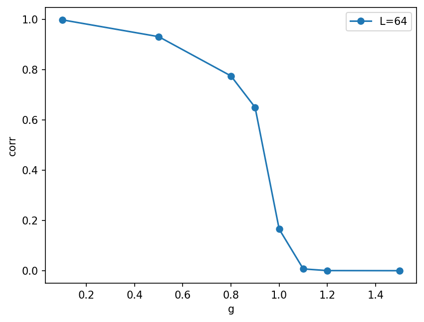
key = 'corr'

plt.figure()
for L in results_all:
    res_L = results_all[L]
    plt.plot(res_L['g'], res_L[key], marker='o', label="L={L:d}".format(L=L))
plt.xlabel('g')
plt.ylabel(key)
plt.legend(loc='best')

<matplotlib.legend.Legend at 0x7f377c808dc0>

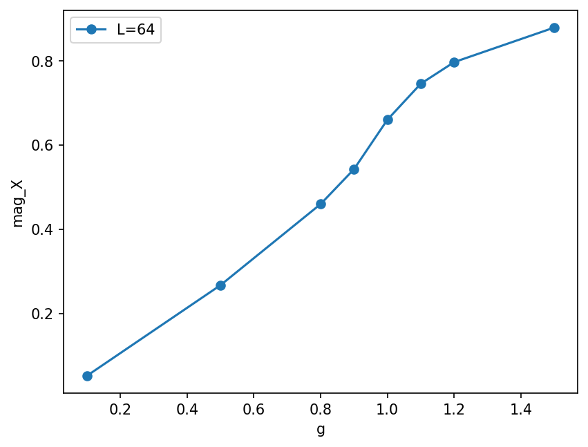
key = 'mag_X'

plt.figure()
for L in results_all:
    res_L = results_all[L]
    plt.plot(res_L['g'], res_L[key], marker='o', label="L={L:d}".format(L=L))
plt.xlabel('g')
plt.ylabel(key)
plt.legend(loc='best')

<matplotlib.legend.Legend at 0x7f3774685510>

key = 'mag_Z'

plt.figure()
for L in results_all:
    res_L = results_all[L]
    plt.plot(res_L['g'], res_L[key], marker='o', label="L={L:d}".format(L=L))
plt.xlabel('g')
plt.ylabel(key)
plt.legend(loc='best')

<matplotlib.legend.Legend at 0x7f37742dd120>

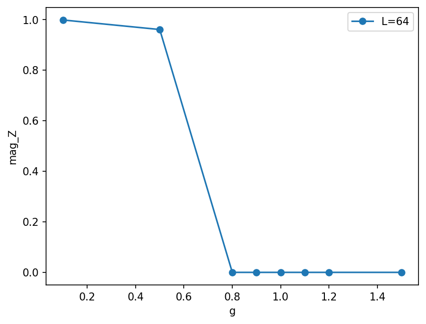
You might wonder what is going on in the plot of mag_Z above in the ferromagnetic phase g < J. In this phase, the system spontaneoulsy breaks the symmetry in the thermodynamic limit, with two ground states $ \lvert `Z :nbsphinx-math:approx :nbsphinx-math:pm 1`:nbsphinx-math:rangle`$. In the finite systems, there is a small splitting into the symmetric and anti-symmetric superpositions $:nbsphinx-math:lvert Z :nbsphinx-math:approx 1` \rangle `:nbsphinx-math:pm :nbsphinx-math:lvert Z :nbsphinx-math:approx -1` \rangle `$ ("cat states"), so that the true finite-L ground state has :math:langle Zrangle = 0`. However, for larger \(L\), this splitting can no longer be resolved, and DMRG breaks the symmetry since this lowers energy due to a smaller truncation error - a cat state needs significantly larger bond dimensions at the same precision.

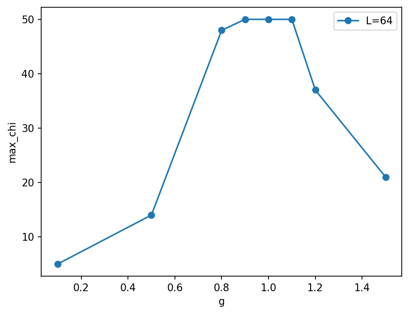
key = 'max_chi'

plt.figure()
for L in results_all:
    res_L = results_all[L]
    plt.plot(res_L['g'], res_L[key], marker='o', label="L={L:d}".format(L=L))
plt.xlabel('g')
plt.ylabel(key)
plt.legend(loc='best')

<matplotlib.legend.Legend at 0x7f37743555d0>

Infinite DMRG

The given DMRG code also works with bc='infinite' boundary conditions of the model and state. The given SimpleDMRG code also allows to run infinite DMRG, simply by replacing the bc='finite' for both the model and the MPS.

• Look at the implementation of d_dmrg.py (and a_mps.py) to see where the differences are.

Again, we can compare to analytic calculations possible for the Transverse Field Ising model.

from tenpy_toycodes.tfi_exact import infinite_gs_energy

The L parameter now just indices the number of tensors insite the unit cell of the infinite MPS. It has to be at least 2, since we optimize 2 tensors at once in our DMRG code. Note that we now use the mean to calculate densities of observables instead of extensive quantities:

model = TFIModel(L=2, J=1., g=0.8, bc='infinite')  # just change bc='infinite' here

chi_max = 10

psi = init_FM_MPS(model.L, model.d, model.bc)
eng = SimpleDMRGEngine(psi, model, chi_max=chi_max, eps=1.e-7)
for i in range(10):
    E_dmrg = eng.sweep()
    E = np.mean(psi.bond_expectation_value(model.H_bonds))
    print("sweep {i:2d}: E/L = {E:.13f}".format(i=i + 1, E=E))
print("final bond dimensions: ", psi.get_chi())
mag_x = np.mean(psi.site_expectation_value(model.sigmax))
mag_z = np.mean(psi.site_expectation_value(model.sigmaz))
print("magnetization density in X = {mag_x:.5f}".format(mag_x=mag_x))
print("magnetization density in Z = {mag_z:.5f}".format(mag_z=mag_z))
E_exact = infinite_gs_energy(model.J, model.g)
print("err in energy = {err:.3e}".format(err=E - E_exact))

sweep  1: E/L = -1.1691320258028
sweep  2: E/L = -1.1859218684668
sweep  3: E/L = -1.1830439651388
sweep  4: E/L = -1.1768668631138
sweep  5: E/L = -1.1725334866568
sweep  6: E/L = -1.1700487255459
sweep  7: E/L = -1.1688086884548
sweep  8: E/L = -1.1682394025940
sweep  9: E/L = -1.1679905285657
sweep 10: E/L = -1.1678847922595
final bond dimensions:  [10, 10]
magnetization density in X = 0.44415
magnetization density in Z = -0.00000
err in energy = -7.528e-05

Exercise: Infinite DMRG

Try running the infinite DMRG code. How many sweeps do you now need to perform to converge now? Does it depend on g and chi?

model = TFIModel(L=2, J=1., g=0.8, bc='infinite')  # just change bc='infinite' here

chi_max = 10

psi = init_FM_MPS(model.L, model.d, model.bc)
eng = SimpleDMRGEngine(psi, model, chi_max=chi_max, eps=1.e-7)
for i in range(100):
    E_dmrg = eng.sweep()
    E = np.mean(psi.bond_expectation_value(model.H_bonds))
    if i % 10 == 9:
        print("sweep {i:2d}: E/L = {E:.13f}".format(i=i + 1, E=E))
print("final bond dimensions: ", psi.get_chi())
mag_x = np.mean(psi.site_expectation_value(model.sigmax))
mag_z = np.mean(psi.site_expectation_value(model.sigmaz))
print("magnetization density in X = {mag_x:.5f}".format(mag_x=mag_x))
print("magnetization density in Z = {mag_z:.5f}".format(mag_z=mag_z))
E_exact = infinite_gs_energy(model.J, model.g)
print("err in energy = {err:.3e}".format(err=E - E_exact))

sweep 10: E/L = -1.1678847922595
sweep 20: E/L = -1.1678095166355
sweep 30: E/L = -1.1678581030541
sweep 40: E/L = -1.1678095085625
sweep 50: E/L = -1.1678095085207
sweep 60: E/L = -1.1678095085207
sweep 70: E/L = -1.1678095085207
sweep 80: E/L = -1.1678095085207
sweep 90: E/L = -1.1678095085207
sweep 100: E/L = -1.1678095085207
final bond dimensions:  [10, 10]
magnetization density in X = 0.44407
magnetization density in Z = 0.88011
err in energy = -6.994e-14

model = TFIModel(L=2, J=1., g=1.0, bc='infinite')  # just change bc='infinite' here

chi_max = 10

psi = init_FM_MPS(model.L, model.d, model.bc)
eng = SimpleDMRGEngine(psi, model, chi_max=chi_max, eps=1.e-7)
for i in range(100):
    E_dmrg = eng.sweep()
    E = np.mean(psi.bond_expectation_value(model.H_bonds))
    if i % 10 == 9:
        print("sweep {i:2d}: E/L = {E:.13f}".format(i=i + 1, E=E))
print("final bond dimensions: ", psi.get_chi())
mag_x = np.mean(psi.site_expectation_value(model.sigmax))
mag_z = np.mean(psi.site_expectation_value(model.sigmaz))
print("magnetization density in X = {mag_x:.5f}".format(mag_x=mag_x))
print("magnetization density in Z = {mag_z:.5f}".format(mag_z=mag_z))
E_exact = infinite_gs_energy(model.J, model.g)
print("err in energy = {err:.3e}".format(err=E - E_exact))

sweep 10: E/L = -1.2734731285873
sweep 20: E/L = -1.2732892142506
sweep 30: E/L = -1.2732583617401
sweep 40: E/L = -1.2732481551659
sweep 50: E/L = -1.2732435768774
sweep 60: E/L = -1.2732411321859
sweep 70: E/L = -1.2732396732724
sweep 80: E/L = -1.2732387344249
sweep 90: E/L = -1.2732380971634
sweep 100: E/L = -1.2732376474834
final bond dimensions:  [10, 10]
magnetization density in X = 0.63816
magnetization density in Z = 0.00000
err in energy = 1.897e-06

From the exercise, you should see that you need significantly more sweeps when the correlation length gets larger, in particular at the critical point! At the critical point, the correlation length (of infinite MPS) scales as \(\xi \propto \chi^\kappa\), so you again need more sweeps to converge at larger bond dimensions.

Advanced exercises for the experts (and those who want to become them ;-) )

• Obtain the ground state of the transverse field ising model at the critical point with DMRG for large L. Try to plot the corrlation function as a function of j-i. What form does it have? Is an MPS a good ansatz for that?

# At the critical point, correlations decay like a power law.
# An MPS can only approximate powerlaws by sums of (decaying) exponentials,
# that decay too fast at long distances.
# In practice, increasing the bond dimension allows to approximate the power laws better and better, so one can still use DMRG.

• Compare running DMRG and imaginary time evolution with TEBD from tenpy_toycodes/c_tebd.py for various parameters of L, J, g, and bc. Which one is faster? Do they always agree?

# imaginary time evolution is significantly slower than the variational DMRG ansatz
# They can give different results e.g. in the symmetry broken phase,
# where TEBD might return a symmetric superposition (cat state),
# while DMRG tends to break the symmetries.