Lattice

full name: tenpy.models.lattice.Lattice
parent module: tenpy.models.lattice
type: class

Inheritance Diagram

Methods

`Lattice.__init__`(Ls, unit_cell[, order, bc, ...])
`Lattice.copy`()	Shallow copy of self.
`Lattice.count_neighbors`([u, key])	Count e.g. the number of nearest neighbors for a site in the bulk.
`Lattice.coupling_shape`(dx)	Calculate correct shape of the strengths for a coupling.
`Lattice.distance`(u1, u2, dx)	Get the distance for a given coupling between two sites in the lattice.
`Lattice.enlarge_mps_unit_cell`([factor])	Repeat the unit cell for infinite MPS boundary conditions; in place.
`Lattice.extract_segment`([first, last, enlarge])	Extract a finite segment from an infinite/large system.
`Lattice.find_coupling_pairs`([max_dx, ...])	Automatically find coupling pairs grouped by distances.
`Lattice.from_hdf5`(hdf5_loader, h5gr, subpath)	Load instance from a HDF5 file.
`Lattice.lat2mps_idx`(lat_idx)	Translate lattice indices `(x_0, ..., x_{D-1}, u)` to MPS index i.
`Lattice.mps2lat_idx`(i)	Translate MPS index i to lattice indices `(x_0, ..., x_{dim-1}, u)`.
`Lattice.mps2lat_values`(A[, axes, u])	Reshape/reorder A to replace an MPS index by lattice indices.
`Lattice.mps2lat_values_masked`(A[, axes, ...])	Reshape/reorder an array A to replace an MPS index by lattice indices.
`Lattice.mps_idx_fix_u`([u])	return an index array of MPS indices for which the site within the unit cell is u.
`Lattice.mps_lat_idx_fix_u`([u])	Similar as `mps_idx_fix_u()`, but return also the corresponding lattice indices.
`Lattice.mps_sites`()	Return a list of sites for all MPS indices.
`Lattice.multi_coupling_shape`(dx)	Calculate correct shape of the strengths for a multi_coupling.
`Lattice.ordering`(order)	Provide possible orderings of the N lattice sites.
`Lattice.plot_basis`(ax[, origin, shade])	Plot arrows indicating the basis vectors of the lattice.
`Lattice.plot_bc_identified`(ax[, direction, ...])	Mark two sites identified by periodic boundary conditions.
`Lattice.plot_brillouin_zone`(ax, args, *kwargs)	Plot the Brillouin Zone of the lattice.
`Lattice.plot_coupling`(ax[, coupling, wrap])	Plot lines connecting nearest neighbors of the lattice.
`Lattice.plot_order`(ax[, order, textkwargs])	Plot a line connecting sites in the specified "order" and text labels enumerating them.
`Lattice.plot_reciprocal_basis`(ax[, origin, ...])	Plot arrows indicating the basis vectors of the reciprocal lattice.
`Lattice.plot_sites`(ax[, markers, labels])	Plot the sites of the lattice with markers.
`Lattice.position`(lat_idx)	return 'space' position of one or multiple sites.
`Lattice.possible_couplings`(u1, u2, dx[, ...])	Find possible MPS indices for two-site couplings.
`Lattice.possible_multi_couplings`(ops[, strength])	Generalization of `possible_couplings()` to couplings with more than 2 sites.
`Lattice.save_hdf5`(hdf5_saver, h5gr, subpath)	Export self into a HDF5 file.
`Lattice.site`(i)	return `Site` instance corresponding to an MPS index i
`Lattice.test_sanity`()	Sanity check.

Class Attributes and Properties

`Lattice.BZ`	The Brillouin Zone as `SimpleBZ`
`Lattice.Lu`	the (expected) number of sites in the unit cell, `len(unit_cell)`.
`Lattice.basis`
`Lattice.boundary_conditions`	Human-readable list of boundary conditions from `bc` and `bc_shift`.
`Lattice.cylinder_axis`	Direction of the cylinder axis.
`Lattice.dim`	the dimension of the lattice
`Lattice.order`	Defines an ordering of the lattice sites, thus mapping the lattice to a 1D chain.
`Lattice.reciprocal_basis`	Reciprocal basis vectors of the lattice.

class tenpy.models.lattice.Lattice(Ls, unit_cell, order='default', bc='open', bc_MPS='finite', basis=None, positions=None, pairs=None)[source]

Bases: object

A general, regular lattice.

The lattice consists of a unit cell which is repeated in dim different directions. A site of the lattice is thus identified by lattice indices (x_0, ..., x_{dim-1}, u), where 0 <= x_l < Ls[l] pick the position of the unit cell in the lattice and 0 <= u < len(unit_cell) picks the site within the unit cell. The site is located in ‘space’ at sum_l x_l*basis[l] + unit_cell_positions[u] (see position()). (Note that the position in space is only used for plotting, not for defining the couplings.)

In addition to the pure geometry, this class also defines an order of all sites. This order maps the lattice to a finite 1D chain and defines the geometry of MPSs and MPOs. The MPS index i corresponds thus to the lattice sites given by (x_0, ..., x_{dim-1}, u) = tuple(self.order[i]). Infinite boundary conditions of the MPS repeat in the first spatial direction of the lattice, i.e., if the site at (x_0, x_1, ..., x_{dim-1},u) has MPS index i, the site at (x_0 + Ls[0], x_1, ..., x_{dim-1}, u) corresponds to MPS index i + N_sites. Use mps2lat_idx() and lat2mps_idx() for conversion of indices. The function mps2lat_values() performs the necessary reshaping and re-ordering from arrays indexed in MPS form to arrays indexed in lattice form.

Parameters:

Ls (list of int) – the length in each direction
unit_cell (list of Site) – The sites making up a unit cell of the lattice. If you want to specify it only after initialization, use None entries in the list.
order (str | ('standard', snake_winding, priority) | ('grouped', groups, ...)) – A string or tuple specifying the order, given to ordering().
bc ((iterable of) {'open' | 'periodic' | int}) – Boundary conditions in each direction of the lattice. A single string holds for all directions. An integer shift means that we have periodic boundary conditions along this direction, but shift/tilt by -shift*lattice.basis[0] (~cylinder axis for bc_MPS='infinite') when going around the boundary along this direction.
bc_MPS ('finite' | 'segment' | 'infinite') – Boundary conditions for an MPS/MPO living on the ordered lattice. If the system is 'infinite', the infinite direction is always along the first basis vector (justifying the definition of N_rings and N_sites_per_ring).
basis (iterable of 1D arrays) – For each direction one translation vectors shifting the unit cell. Defaults to the standard ONB np.eye(dim).
positions (iterable of 1D arrays) – For each site of the unit cell the position within the unit cell. Defaults to np.zeros((len(unit_cell), dim)).
pairs (dict) – Of the form {'nearest_neighbors': [(u1, u2, dx), ...], ...}. Typical keys are 'nearest_neighbors', 'next_nearest_neighbors'. For each of them, it specifies a list of tuples (u1, u2, dx) which can be used as parameters for add_coupling() to generate couplings over each pair of ,e.g., 'nearest_neighbors'. Note that this adds couplings for each pair only in one direction!

Ls

the length in each direction.

Type:: tuple of int

shape

the ‘shape’ of the lattice, same as Ls + (len(unit_cell), )

Type:: tuple of int

N_cells

the number of unit cells in the lattice, np.prod(self.Ls).

Type:: int

N_sites

the number of sites in the lattice, np.prod(self.shape).

Type:: int

N_sites_per_ring

Defined as N_sites / Ls[0], for an infinite system the number of sites per “ring”.

Type:: int

N_rings

Alias for Ls[0], for an infinite system the number of “rings” in the unit cell.

Type:: int

unit_cell

the sites making up a unit cell of the lattice.

Type:: list of Site

bc

Boundary conditions of the couplings in each direction of the lattice, translated into a bool array with the global bc_choices.

Type:: bool ndarray

bc_shift

The shift in x-direction when going around periodic boundaries in other directions; entries for [y, z, …]; length is dim - 1

Type:: None | ndarray(int)

bc_MPS

Boundary conditions for an MPS/MPO living on the ordered lattice. If the system is 'infinite', the infinite direction is always along the first basis vector (justifying the definition of N_rings and N_sites_per_ring).

Type:: ‘finite’ | ‘segment’ | ‘infinite’

basis

translation vectors shifting the unit cell. The row i gives the vector shifting in direction i.

Type:: ndarray (dim, Dim)

unit_cell_positions

for each site in the unit cell a vector giving its position within the unit cell.

Type:: ndarray, shape (len(unit_cell), Dim)

position_disorder

If None (default) the lattice positions are regular. If not None, this array specifies a shift of each site relative to the regular lattice, possibly introducing a disorder of each site. It is only used by position() (e.g. when plotting lattice sites) and distance(). To use this, you can set the position_disorder in a model, and then read out and use the distance() to possibly rescale the coupling strengths. The correct shape is Ls[0], Ls[1], ..., len(unit_cell), Dim, where Dim is the same dimension as for the unit_cell_positions and basis.

Type:: None | ndarray

pairs

See above.

Type:: dict

segment_first_last

The first and last MPS sites for “segment” bc_MPS; not set otherwise.

Type:: tuple of int

_order

The place where order is stored.

Type:: ndarray (N_sites, dim+1)

_strides

necessary for lat2mps_idx().

Type:: ndarray (dim, )

_perm

permutation needed to make order lexsorted, _perm = np.lexsort(_order.T).

Type:: ndarray (N, )

_mps2lat_vals_idx

index array for reshape/reordering in mps2lat_vals()

Type:: ndarray shape

_mps_fix_u

for each site of the unit cell an index array selecting the mps indices of that site.

Type:: tuple of ndarray (N_cells, ) np.intp

_mps2lat_vals_idx_fix_u

similar as _mps2lat_vals_idx, but for a fixed u picking a site from the unit cell.

Type:: tuple of ndarray of shape Ls

Lu = None: the (expected) number of sites in the unit cell, len(unit_cell).

test_sanity()[source]

Sanity check.

Raises ValueErrors, if something is wrong.

copy()[source]: Shallow copy of self.

save_hdf5(hdf5_saver, h5gr, subpath)[source]

Export self into a HDF5 file.

This method saves all the data it needs to reconstruct self with from_hdf5().

Specifically, it saves unit_cell, Ls, unit_cell_positions, basis, boundary_conditions, pairs under their name, bc_MPS as "boundary_conditions_MPS", and order as "order_for_MPS". Moreover, it saves dim and N_sites as HDF5 attributes.

Parameters:

hdf5_saver (Hdf5Saver) – Instance of the saving engine.
h5gr (:class`Group`) – HDF5 group which is supposed to represent self.
subpath (str) – The name of h5gr with a '/' in the end.

classmethod from_hdf5(hdf5_loader, h5gr, subpath)[source]

Load instance from a HDF5 file.

This method reconstructs a class instance from the data saved with save_hdf5().

Parameters:

hdf5_loader (Hdf5Loader) – Instance of the loading engine.
h5gr (Group) – HDF5 group which is representing the object to be constructed.
subpath (str) – The name of h5gr with a '/' in the end.

Returns:

obj – Newly generated class instance containing the required data.

Return type:

cls

property dim: the dimension of the lattice

property order

Defines an ordering of the lattice sites, thus mapping the lattice to a 1D chain.

Each row of the array contains the lattice indices for one site, the order of the rows thus specifies a path through the lattice, along which an MPS will wind through the lattice.

You can visualize the order with plot_order().

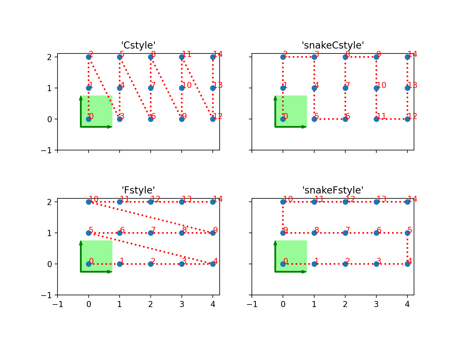
ordering(order)[source]

Provide possible orderings of the N lattice sites.

Subclasses often override this function to define additional orderings.

Possible strings for the order defined here are:

'Cstyle', 'default' :
Recommended in most cases. First within the unit cell, then along y, then x. priority=(0, 1, ..., dim-1, dim).

'snake', 'snakeCstyle' :
Back and forth along the various directions, in Cstyle priority. Equivalent to snake_winding=(True, ..., True, True) and priority=(0, 1, ..., dim-1, dim).

'Fstyle' :
Might be good for almost completely decoupled chains in a finite, long ladder/cylinder; in other cases not a good idea. Equivalent to snake_winding=(False, ..., False, False) and priority=(dim-1, ..., 1., 0, dim).

'snakeFstyle' :
Snake-winding for Fstyle. Equivalent to snake_winding=(True, ..., True, True) and priority=(dim-1, ..., 1., 0, dim).

(Source code, png, hires.png, pdf)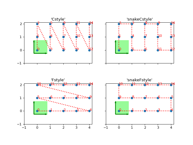

../_images/tenpy-models-lattice-Lattice-1.png

Note

For lattices with a non-trivial unit cell (e.g. Honeycomb, Kagome), the grouped order might be more appropriate, see get_order_grouped().

Parameters:: order (str | ('standard', snake_winding, priority) | ('grouped', groups, ...)) – Specifies the desired ordering using one of the strings of the above tables. Alternatively, an ordering is specified by a tuple with first entry specifying a function, 'standard' for get_order() and 'grouped' for get_order_grouped(), and other arguments in the tuple as specified in the documentation of these functions.
Returns:: order – the order to be used for order.
Return type:: array, shape (N, D+1), dtype np.intp

See also

get_order: generates the order from equivalent priority and snake_winding.
get_order_grouped: variant of get_order.
plot_order: visualizes the resulting order.

property boundary_conditions

Human-readable list of boundary conditions from bc and bc_shift.

Returns:: boundary_conditions – List of "open" or "periodic", one entry for each direction of the lattice.
Return type:: list of str

property cylinder_axis

Direction of the cylinder axis.

For an infinite cylinder (bc_MPS=’infinite’ and ``boundary_conditions[1] == ‘open’`), this property gives the direction of the cylinder axis, in the same coordinates as the basis, as a normalized vector. For a 1D lattice or for open boundary conditions along y, it’s just along basis[0].

extract_segment(first=0, last=None, enlarge=None)[source]

Extract a finite segment from an infinite/large system.

Parameters:

first (int) – The first and last site to include into the segment. last defaults to L - 1, i.e., the MPS unit cell for infinite MPS.
last (int) – The first and last site to include into the segment. last defaults to L - 1, i.e., the MPS unit cell for infinite MPS.
enlarge (int) – Instead of specifying the first and last site, you can specify this factor by how much the MPS unit cell should be enlarged.

Returns:

copy – A copy of self with “segment” bc_MPS and segment_first_last set.

Return type:

Lattice

enlarge_mps_unit_cell(factor=2)[source]

Repeat the unit cell for infinite MPS boundary conditions; in place.

Parameters:: factor (int) – The new number of sites in the MPS unit cell will be increased from N_sites to factor*N_sites_per_ring. Since MPS unit cells are repeated in the x-direction in our convention, the lattice shape goes from (Lx, Ly, ..., Lu) to (Lx*factor, Ly, ..., Lu).

position(lat_idx)[source]

return ‘space’ position of one or multiple sites.

Parameters:: lat_idx (ndarray, (... , dim+1)) – Lattice indices.
Returns:: pos – The position of the lattice sites specified by lat_idx in real-space. If position_disorder is non-trivial, it can shift the positions!
Return type:: ndarray, (..., Dim)

site(i)[source]: return Site instance corresponding to an MPS index i

mps_sites()[source]

Return a list of sites for all MPS indices.

Equivalent to [self.site(i) for i in range(self.N_sites)].

This should be used for sites of 1D tensor networks (MPS, MPO,…).

mps2lat_idx(i)[source]

Translate MPS index i to lattice indices (x_0, ..., x_{dim-1}, u).

Parameters:: i (int | array_like of int) – MPS index/indices.
Returns:: lat_idx – First dimensions like i, last dimension has len dim`+1 and contains the lattice indices ``(x_0, …, x_{dim-1}, u)` corresponding to i. For i across the MPS unit cell and “infinite” or “segment” bc_MPS, we shift x_0 accordingly.
Return type:: array

lat2mps_idx(lat_idx)[source]

Translate lattice indices (x_0, ..., x_{D-1}, u) to MPS index i.

Parameters:: lat_idx (array_like [..., dim+1]) – The last dimension corresponds to lattice indices (x_0, ..., x_{D-1}, u). All lattice indices should be positive and smaller than the corresponding entry in self.shape. Exception: for “infinite” or “segment” bc_MPS, an x_0 outside indicates shifts across the boundary.
Returns:: i – MPS index/indices corresponding to lat_idx. Has the same shape as lat_idx without the last dimension.
Return type:: array_like

mps_idx_fix_u(u=None)[source]

return an index array of MPS indices for which the site within the unit cell is u.

If you have multiple sites in your unit-cell, an onsite operator is in general not defined for all sites. This functions returns an index array of the mps indices which belong to sites given by self.unit_cell[u].

Parameters:: u (None | int) – Selects a site of the unit cell. None (default) means all sites.
Returns:: mps_idx – MPS indices for which self.site(i) is self.unit_cell[u]. Ordered ascending.
Return type:: array

mps_lat_idx_fix_u(u=None)[source]

Similar as mps_idx_fix_u(), but return also the corresponding lattice indices.

Parameters:

u (None | int) – Selects a site of the unit cell. None (default) means all sites.

Returns:

mps_idx (array) – MPS indices i for which self.site(i) is self.unit_cell[u].
lat_idx (2D array) – The row j contains the lattice index (without u) corresponding to mps_idx[j].

mps2lat_values(A, axes=0, u=None)[source]

Reshape/reorder A to replace an MPS index by lattice indices.

Parameters:

A (ndarray) – Some values. Must have A.shape[axes] = self.N_sites if u is None, or A.shape[axes] = self.N_cells if u is an int.
axes ((iterable of) int) – chooses the axis which should be replaced.
u (None | int) – Optionally choose a subset of MPS indices present in the axes of A, namely the indices corresponding to self.unit_cell[u], as returned by mps_idx_fix_u(). The resulting array will not have the additional dimension(s) of u.

Returns:

res_A – Reshaped and reordered version of A. Such that MPS indices along the specified axes are replaced by lattice indices, i.e., if MPS index j maps to lattice site (x0, x1, x2), then res_A[..., x0, x1, x2, ...] = A[..., j, ...].

Return type:

ndarray

Examples

Say you measure expectation values of an onsite term for an MPS, which gives you an 1D array A, where A[i] is the expectation value of the site given by self.mps2lat_idx(i). Then this function gives you the expectation values ordered by the lattice:

>>> print(lat.shape, A.shape)
(10, 3, 2) (60,)
>>> A_res = lat.mps2lat_values(A)
>>> A_res.shape
(10, 3, 2)
>>> bool(A_res[tuple(lat.mps2lat_idx(5))] == A[5])
True

If you have a correlation function C[i, j], it gets just slightly more complicated:

>>> print(lat.shape, C.shape)
(10, 3, 2) (60, 60)
>>> lat.mps2lat_values(C, axes=[0, 1]).shape
(10, 3, 2, 10, 3, 2)

If the unit cell consists of different physical sites, an onsite operator might be defined only on one of the sites in the unit cell. Then you can use mps_idx_fix_u() to get the indices of sites it is defined on, measure the operator on these sites, and use the argument u of this function.

>>> u = 0
>>> idx_subset = lat.mps_idx_fix_u(u)
>>> A_u = A[idx_subset]
>>> A_u_res = lat.mps2lat_values(A_u, u=u)
>>> A_u_res.shape
(10, 3)
>>> bool(np.all(A_res[:, :, u] == A_u_res[:, :]))
True

mps2lat_values_masked(A, axes=-1, mps_inds=None, include_u=None)[source]

Reshape/reorder an array A to replace an MPS index by lattice indices.

This is a generalization of mps2lat_values() allowing for the case of an arbitrary set of MPS indices present in each axis of A.

Parameters:

A (ndarray) – Some values.
axes ((iterable of) int) – Chooses the axis of A which should be replaced. If multiple axes are given, you also need to give multiple index arrays as mps_inds.
mps_inds ((list of) 1D ndarray) – Specifies for each axis in axes, for which MPS indices we have values in the corresponding axis of A. Defaults to [np.arange(A.shape[ax]) for ax in axes]. For indices across the MPS unit cell and “infinite” bc_MPS, we shift x_0 accordingly.
include_u ((list of) bool) – Specifies for each axis in axes, whether the u index of the lattice should be included into the output array res_A. Defaults to len(self.unit_cell) > 1.

Returns:

res_A – Reshaped and reordered copy of A. Such that MPS indices along the specified axes are replaced by lattice indices, i.e., if MPS index j maps to lattice site (x0, x1, x2), then res_A[..., x0, x1, x2, ...] = A[..., mps_inds[j], ...].

Return type:

np.ma.MaskedArray

count_neighbors(u=0, key='nearest_neighbors')[source]

Count e.g. the number of nearest neighbors for a site in the bulk.

Parameters:

u (int) – Specifies the site in the unit cell, for which we should count the number of neighbors (or whatever key specifies).
key (str) – Key of pairs to select what to count.

Returns:

number – Number of nearest neighbors (or whatever key specified) for the u-th site in the unit cell, somewhere in the bulk of the lattice. Note that it might not be the correct value at the edges of a lattice with open boundary conditions.

Return type:

int

distance(u1, u2, dx)[source]

Get the distance for a given coupling between two sites in the lattice.

The u1, u2, dx parameters are defined in analogy with add_coupling(), i.e., this function calculates the distance between a pair of operators added with add_coupling (using the basis and unit_cell_positions of the lattice).

Warning

This function ignores “wrapping” around the cylinder in the case of periodic boundary conditions.

Parameters:

u1 (int) – Indices within the unit cell; the u1 and u2 of add_coupling()
u2 (int) – Indices within the unit cell; the u1 and u2 of add_coupling()
dx (array) – Length dim. The translation in terms of basis vectors for the coupling.

Returns:

distance – The distance between site at lattice indices [x, y, u1] and [x + dx[0], y + dx[1], u2], ignoring any boundary effects. In case of non-trivial position_disorder, an array is returned. This array is compatible with the shape/indexing required for add_coupling(). For example to add a Z-Z interaction of strength J/r with r the distance, you can do something like this in init_terms():

for u1, u2, dx in self.lat.pairs[‘nearest_neighbors’]:
dist = self.lat.distance(u1, u2, dx) self.add_coupling(J/dist, u1, ‘Sz’, u2, ‘Sz’, dx)

Return type:

float | ndarray

find_coupling_pairs(max_dx=3, cutoff=None, eps=1e-10)[source]

Automatically find coupling pairs grouped by distances.

Given the unit_cell_positions and basis, the coupling pairs of nearest_neighbors, next_nearest_neighbors etc at a given distance are basically fixed (although not uniquely, since we take out half of them to avoid double-counting couplings in both directions A_i B_j + B_i A_i). This function iterates through all possible couplings up to a given cutoff distance and then determines the possible pairs at fixed distances (up to round-off errors).

Parameters:

max_dx (int) – Maximal index for each index of dx to iterate over. You need large enough values to include every possible coupling up to the desired distance, but choosing it too large might make this function run for a long time.
cutoff (float) – Maximal distance (in the units in which basis and unit_cell_positions is given).
eps (float) – Tolerance up to which to distances are considered the same.

Returns:

coupling_pairs – Keys are distances of nearest-neighbors, next-nearest-neighbors etc. Values are [(u1, u2, dx), ...] as in pairs.

Return type:

dict

coupling_shape(dx)[source]

Calculate correct shape of the strengths for a coupling.

Parameters:

dx (tuple of int) – Translation vector in the lattice for a coupling of two operators. Corresponds to dx argument of tenpy.models.model.CouplingModel.add_multi_coupling().

Returns:

coupling_shape (tuple of int) – Len dim. The correct shape for an array specifying the coupling strength. lat_indices has only rows within this shape.
shift_lat_indices (array) – Translation vector from origin to the lower left corner of box spanned by dx.

possible_couplings(u1, u2, dx, strength=None)[source]

Find possible MPS indices for two-site couplings.

For periodic boundary conditions (bc[a] == False) the index x_a is taken modulo Ls[a] and runs through range(Ls[a]). For open boundary conditions, x_a is limited to 0 <= x_a < Ls[a] and 0 <= x_a+dx[a] < lat.Ls[a].

Parameters:

u1 (int) – Indices within the unit cell; the u1 and u2 of add_coupling()
u2 (int) – Indices within the unit cell; the u1 and u2 of add_coupling()
dx (array) – Length dim. The translation in terms of basis vectors for the coupling.
strength (array_like | None) – If given, instead of returning lat_indices and coupling_shape directly return the correct strength_12.

Returns:

mps1, mps2 (1D array) – For each possible two-site coupling the MPS indices for the u1 and u2.
strength_vals (1D array) – (Only returned if strength is not None.) Such that for (i, j, s) in zip(mps1, mps2, strength_vals): iterates over all possible couplings with s being the strength of that coupling. Couplings where strength_vals == 0. are filtered out.
lat_indices (2D int array) – (Only returned if strength is None.) Rows of lat_indices correspond to entries of mps1 and mps2 and contain the lattice indices of the “lower left corner” of the box containing the coupling.
coupling_shape (tuple of int) – (Only returned if strength is None.) Len dim. The correct shape for an array specifying the coupling strength. lat_indices has only rows within this shape.

multi_coupling_shape(dx)[source]

Calculate correct shape of the strengths for a multi_coupling.

Parameters:

dx (2D array, shape (N_ops, dim)) – dx[i, :] is the translation vector in the lattice for the i-th operator. Corresponds to the dx of each operator given in the argument ops of tenpy.models.model.CouplingModel.add_multi_coupling().

Returns:

coupling_shape (tuple of int) – Len dim. The correct shape for an array specifying the coupling strength. lat_indices has only rows within this shape.
shift_lat_indices (array) – Translation vector from origin to the lower left corner of box spanned by dx. (Unlike for coupling_shape() it can also contain entries > 0)

possible_multi_couplings(ops, strength=None)[source]

Generalization of possible_couplings() to couplings with more than 2 sites.

Parameters:

ops (list of (opname, dx, u)) – Same as the argument ops of add_multi_coupling().

Returns:

mps_ijkl (2D int array) – Each row contains MPS indices i,j,k,l,…` for each of the operators positions. The positions are defined by dx (j,k,l,… relative to i) and boundary conditions of self (how much the box for given dx can be shifted around without hitting a boundary - these are the different rows).
strength_vals (1D array) – (Only returned if strength is not None.) Such that for (ijkl, s) in zip(mps_ijkl, strength_vals): iterates over all possible couplings with s being the strength of that coupling. Couplings where strength_vals == 0. are filtered out.
lat_indices (2D int array) – (Only returned if strength is None.) Rows of lat_indices correspond to rows of mps_ijkl and contain the lattice indices of the “lower left corner” of the box containing the coupling.
coupling_shape (tuple of int) – (Only returned if strength is None.) Len dim. The correct shape for an array specifying the coupling strength. lat_indices has only rows within this shape.

plot_sites(ax, markers=['o', '^', 's', 'p', 'h', 'D'], labels=None, **kwargs)[source]

Plot the sites of the lattice with markers.

Parameters:

ax (matplotlib.axes.Axes) – The axes on which we should plot.
markers (list) – List of values for the keyword marker of ax.plot() to distinguish the different sites in the unit cell, a site u in the unit cell is plotted with a marker markers[u % len(markers)].
labels (list of str) – Labels for the different sites in the unit cell.
**kwargs – Further keyword arguments given to ax.plot().

plot_order(ax, order=None, textkwargs={'color': 'r'}, **kwargs)[source]

Plot a line connecting sites in the specified “order” and text labels enumerating them.

Parameters:

ax (matplotlib.axes.Axes) – The axes on which we should plot.
order (None | 2D array (self.N_sites, self.dim+1)) – The order as returned by ordering(); by default (None) use order.
textkwargs (None | dict) – If not None, we add text labels enumerating the sites in the plot. The dictionary can contain keyword arguments for ax.text().
**kwargs – Further keyword arguments given to ax.plot().

plot_coupling(ax, coupling=None, wrap=False, **kwargs)[source]

Plot lines connecting nearest neighbors of the lattice.

Parameters:

ax (matplotlib.axes.Axes) – The axes on which we should plot.
coupling (list of (u1, u2, dx)) – By default (None), use self.pairs['nearest_neighbors']. Specifies the connections to be plotted; iterating over lattice indices (i0, i1, …), we plot a connection from the site (i0, i1, ..., u1) to the site (i0+dx[0], i1+dx[1], ..., u2), taking into account the boundary conditions.
wrap (bool) – If True, plot couplings going around the boundary by directly connecting the sites it connects. This might be hard to see, as this puts lines from one end of the lattice to the other. If False, plot the couplings as dangling lines.
**kwargs – Further keyword arguments given to ax.plot().

plot_basis(ax, origin=(0.0, 0.0), shade=None, **kwargs)[source]

Plot arrows indicating the basis vectors of the lattice.

Parameters:

ax (matplotlib.axes.Axes) – The axes on which we should plot.
**kwargs – Keyword arguments for ax.arrow.

plot_reciprocal_basis(ax, origin=(0.0, 0.0), plot_symmetric=True, **kwargs)[source]

Plot arrows indicating the basis vectors of the reciprocal lattice.

(Same as plot_basis(), but without shading, since Brillouin zone is drawn separately)

Parameters:

ax (matplotlib.axes.Axes) – The axes on which we should plot.
plot_symmetric (bool, default=True) – if True, centers the plot around the origin
origin (iterable) – coordinates of the origin
**kwargs – Keyword arguments for ax.arrow.

plot_bc_identified(ax, direction=-1, origin=None, cylinder_axis=False, **kwargs)[source]

Mark two sites identified by periodic boundary conditions.

Works only for lattice with a 2-dimensional basis.

Parameters:

ax (matplotlib.axes.Axes) – The axes on which we should plot.
direction (int) – The direction of the lattice along which we should mark the identified sites. If None, mark it along all directions with periodic boundary conditions.
cylinder_axis (bool) – Whether to plot the cylinder axis as well.
origin (None | np.ndarray) – The origin starting from where we mark the identified sites. Defaults to the first entry of unit_cell_positions.
**kwargs – Keyword arguments for the used ax.plot.

plot_brillouin_zone(ax, *args, **kwargs)[source]

Plot the Brillouin Zone of the lattice.

Parameters:

ax (matplotlib.axes.Axes) – The axes on which we should plot.
*args – arguments for plot_brillouin_zone() of :class:self.BZ.__class__.
**kwargs – Keyword arguments for plot_brillouin_zone() of :class:self.BZ.__class__.

property reciprocal_basis

Reciprocal basis vectors of the lattice.

The reciprocal basis vectors obey \(a_i b_j = 2 \pi \delta_{i, j}\), such that b_j = reciprocal_basis[j]

property BZ: The Brillouin Zone as SimpleBZ