Chain
full name: tenpy.models.lattice.Chain
parent module:
tenpy.models.latticetype: class
Inheritance Diagram
Methods
|
|
Shallow copy of self. |
|
|
Count e.g. the number of nearest neighbors for a site in the bulk. |
Calculate correct shape of the strengths for a coupling. |
|
|
Get the distance for a given coupling between two sites in the lattice. |
|
Repeat the unit cell for infinite MPS boundary conditions; in place. |
|
Extract a finite segment from an infinite/large system. |
|
Automatically find coupling pairs grouped by distances. |
|
Load instance from a HDF5 file. |
|
Initialize by reading sizes, boundary conditions etc from model_params. |
|
Translate lattice indices |
Translate MPS index i to lattice indices |
|
|
Same as |
|
Reshape/reorder an array A to replace an MPS index by lattice indices. |
|
Return an index array of MPS indices for which the site within the unit cell is u. |
Similar as |
|
Return a list of sites for all MPS indices. |
|
Calculate correct shape of the strengths for a multi_coupling. |
|
|
Provide possible orderings of the N lattice sites. |
|
Plot arrows indicating the basis vectors of the lattice. |
|
Mark two sites identified by periodic boundary conditions. |
|
Plot the Brillouin Zone of the lattice. |
|
Plot lines connecting nearest neighbors of the lattice. |
|
Plot a line connecting sites in the specified "order" and text labels enumerating them. |
|
Plot arrows indicating the basis vectors of the reciprocal lattice. |
|
Plot the sites of the lattice with markers. |
|
Return 'space' position of one or multiple sites. |
|
Find possible MPS indices for two-site couplings. |
|
Generalization of |
|
Export self into a HDF5 file. |
|
Return |
Sanity check. |
|
|
Return a lattice with sites given by grouped_sites. |
Class Attributes and Properties
The Brillouin Zone as |
|
the (expected) number of sites in the unit cell, |
|
|
|
Human-readable list of boundary conditions from |
|
Direction of the cylinder axis. |
|
the dimension of the lattice |
|
Defines an ordering of the lattice sites, thus mapping the lattice to a 1D chain. |
|
Reciprocal basis vectors of the lattice. |
|
|
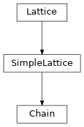
- class tenpy.models.lattice.Chain(L, site, **kwargs)[source]
Bases:
SimpleLatticeA chain of L equal sites.
Defined pairs are
'nearest_neighbors','next_nearest_neighbors', and'next_next_nearest_neighbors'.(
Source code,png,hires.png,pdf)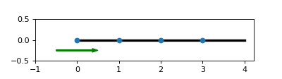
(
Source code,png,hires.png,pdf)
- Parameters:
- dim = 1
the dimension of the lattice
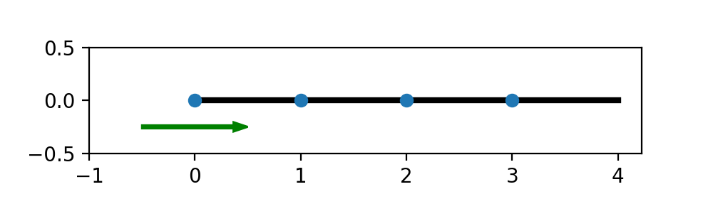
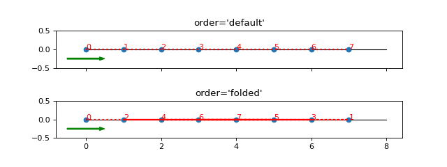
- ordering(order)[source]
Provide possible orderings of the N lattice sites.
The following orders are defined here in addition to
Lattice.ordering():'default':Just along the chain,
0, 1, 2, 3, 4, ... ,L-1.'folded':Yields
0, L-1, 1, L-2, ... , L//2. This order might be useful if you want to consider a ring with periodic boundary conditions with a finite MPS: if you squeeze this ring to a long oval and zig-zag through the top and bottom, you get this order. Thus, it avoids the ultra-long-range coupling from site 0 to L-1, at the expense of (almost) each nearest-neighbor coupling now being next-nearest-neighbors. Graphically:| PBC couplings on ring ---> MPS order='folded' | number=physical site number=position in MPS | | --1---2---3---4 2 4 6 8 | / \ : : : : : : : : | 0 5 ---> 0 : : : : : : : : 10 | : / : : : : : : : : : : | 10--9---8---7-6 1 3 5 7 9
- Lu = 1
the (expected) number of sites in the unit cell,
len(unit_cell).
- property boundary_conditions
Human-readable list of boundary conditions from
bcandbc_shift.- Returns:
boundary_conditions – List of
"open"or"periodic"or integer, one entry for each direction of the lattice. An integer means periodic boundary condition with a shift given by that number, seebc_shift.- Return type:
list of {str | int}
- count_neighbors(u=0, key='nearest_neighbors')[source]
Count e.g. the number of nearest neighbors for a site in the bulk.
- Parameters:
- Returns:
number – Number of nearest neighbors (or whatever key specified) for the u-th site in the unit cell, somewhere in the bulk of the lattice. Note that it might not be the correct value at the edges of a lattice with open boundary conditions.
- Return type:
- coupling_shape(dx)[source]
Calculate correct shape of the strengths for a coupling.
- Parameters:
dx (tuple of int) – Translation vector in the lattice for a coupling of two operators. Corresponds to dx argument of
tenpy.models.model.CouplingModel.add_multi_coupling().- Returns:
coupling_shape (tuple of int) – Len
dim. The correct shape for an array specifying the coupling strength. lat_indices has only rows within this shape.shift_lat_indices (array) – Translation vector from origin to the lower left corner of box spanned by dx.
- property cylinder_axis
Direction of the cylinder axis.
For an infinite cylinder (bc_MPS=’infinite’ and ``boundary_conditions[1] == ‘open’`), this property gives the direction of the cylinder axis, in the same coordinates as the
basis, as a normalized vector. For a 1D lattice or for open boundary conditions along y, it’s just alongbasis[0].
- distance(u1, u2, dx)[source]
Get the distance for a given coupling between two sites in the lattice.
The u1, u2, dx parameters are defined in analogy with
add_coupling(), i.e., this function calculates the distance between a pair of operators added with add_coupling (using thebasisandunit_cell_positionsof the lattice).Warning
This function ignores “wrapping” around the cylinder in the case of periodic boundary conditions.
- Parameters:
u1 (int) – Indices within the unit cell; the u1 and u2 of
add_coupling()u2 (int) – Indices within the unit cell; the u1 and u2 of
add_coupling()dx (array) – Length
dim. The translation in terms of basis vectors for the coupling.
- Returns:
distance – The distance between site at lattice indices
[x, y, u1]and[x + dx[0], y + dx[1], u2], ignoring any boundary effects. In case of non-trivialposition_disorder, an array is returned. This array is compatible with the shape/indexing required foradd_coupling(). For example to add a Z-Z interaction of strength J/r with r the distance, you can do something like this ininit_terms():- for u1, u2, dx in self.lat.pairs[‘nearest_neighbors’]:
dist = self.lat.distance(u1, u2, dx) self.add_coupling(J/dist, u1, ‘Sz’, u2, ‘Sz’, dx)
- Return type:
float | ndarray
- enlarge_mps_unit_cell(factor=2)[source]
Repeat the unit cell for infinite MPS boundary conditions; in place.
- Parameters:
factor (int) – The new number of sites in the MPS unit cell will be increased from N_sites to
factor*N_sites. Since MPS unit cells are repeated in the x-direction in our convention, the lattice shape goes from(Lx, Ly, ..., Lu)to(Lx*factor, Ly, ..., Lu).
- extract_segment(first=0, last=None, enlarge=None)[source]
Extract a finite segment from an infinite/large system.
- Parameters:
first (int) – The first and last site to include into the segment. last defaults to
L- 1, i.e., the MPS unit cell for infinite MPS.last (int) – The first and last site to include into the segment. last defaults to
L- 1, i.e., the MPS unit cell for infinite MPS.enlarge (int) – Instead of specifying the first and last site, you can specify this factor by how much the MPS unit cell should be enlarged.
- Returns:
copy – A copy of self with “segment”
bc_MPSandsegment_first_lastset.- Return type:
- find_coupling_pairs(max_dx=3, cutoff=None, eps=1e-10)[source]
Automatically find coupling pairs grouped by distances.
Given the
unit_cell_positionsandbasis, the couplingpairsof nearest_neighbors, next_nearest_neighbors etc at a given distance are basically fixed (although not uniquely, since we take out half of them to avoid double-counting couplings in both directionsA_i B_j + B_i A_i). This function iterates through all possible couplings up to a given cutoff distance and then determines the possiblepairsat fixed distances (up to round-off errors).- Parameters:
max_dx (int) – Maximal index for each index of dx to iterate over. You need large enough values to include every possible coupling up to the desired distance, but choosing it too large might make this function run for a long time.
cutoff (float) – Maximal distance (in the units in which
basisandunit_cell_positionsis given).eps (float) – Tolerance up to which to distances are considered the same.
- Returns:
coupling_pairs – Keys are distances of nearest-neighbors, next-nearest-neighbors etc. Values are
[(u1, u2, dx), ...]as inpairs.- Return type:
- classmethod from_hdf5(hdf5_loader, h5gr, subpath)[source]
Load instance from a HDF5 file.
This method reconstructs a class instance from the data saved with
save_hdf5().- Parameters:
hdf5_loader (
Hdf5Loader) – Instance of the loading engine.h5gr (
Group) – HDF5 group which is representing the object to be constructed.subpath (str) – The name of h5gr with a
'/'in the end.
- Returns:
obj – Newly generated class instance containing the required data.
- Return type:
cls
- classmethod from_model_params(model_params, sites)[source]
Initialize by reading sizes, boundary conditions etc from model_params.
Mainly used during
tenpy.models.model.CouplingMPOModel.init_lattice().
- lat2mps_idx(lat_idx)[source]
Translate lattice indices
(x_0, ..., x_{D-1}, u)to MPS index i.- Parameters:
lat_idx (array_like [..., dim+1]) – The last dimension corresponds to lattice indices
(x_0, ..., x_{D-1}, u). All lattice indices should be positive and smaller than the corresponding entry inself.shape. Exception: for “infinite” or “segment” bc_MPS, an x_0 outside indicates shifts across the boundary.- Returns:
i – MPS index/indices corresponding to lat_idx. Has the same shape as lat_idx without the last dimension.
- Return type:
array_like
- mps2lat_idx(i)[source]
Translate MPS index i to lattice indices
(x_0, ..., x_{dim-1}, u).- Parameters:
- Returns:
lat_idx – First dimensions like i, last dimension has len dim`+1 and contains the lattice indices ``(x_0, …, x_{dim-1}, u)` corresponding to i. For i across the MPS unit cell and “infinite” or “segment” bc_MPS, we shift x_0 accordingly.
- Return type:
array
- mps2lat_values(A, axes=0, u=None)[source]
Same as
Lattice.mps2lat_values(), but ignoreu, setting it to0.
- mps2lat_values_masked(A, axes=-1, mps_inds=None, include_u=None)[source]
Reshape/reorder an array A to replace an MPS index by lattice indices.
This is a generalization of
mps2lat_values()allowing for the case of an arbitrary set of MPS indices present in each axis of A.- Parameters:
A (ndarray) – Some values.
axes ((iterable of) int) – Chooses the axis of A which should be replaced. If multiple axes are given, you also need to give multiple index arrays as mps_inds.
mps_inds ((list of) 1D ndarray) – Specifies for each axis in axes, for which MPS indices we have values in the corresponding axis of A. Defaults to
[np.arange(A.shape[ax]) for ax in axes]. For indices across the MPS unit cell and “infinite” bc_MPS, we shift x_0 accordingly.include_u ((list of) bool) – Specifies for each axis in axes, whether the u index of the lattice should be included into the output array res_A. Defaults to
len(self.unit_cell) > 1.
- Returns:
res_A – Reshaped and reordered copy of A. Such that MPS indices along the specified axes are replaced by lattice indices, i.e., if MPS index j maps to lattice site (x0, x1, x2), then
res_A[..., x0, x1, x2, ...] = A[..., mps_inds[j], ...].- Return type:
np.ma.MaskedArray
- mps_idx_fix_u(u=None)[source]
Return an index array of MPS indices for which the site within the unit cell is u.
If you have multiple sites in your unit-cell, an onsite operator is in general not defined for all sites. This functions returns an index array of the mps indices which belong to sites given by
self.unit_cell[u].- Parameters:
u (None | int) – Selects a site of the unit cell.
None(default) means all sites.- Returns:
mps_idx – MPS indices for which
self.site(i) is self.unit_cell[u]. Ordered ascending.- Return type:
array
- mps_lat_idx_fix_u(u=None)[source]
Similar as
mps_idx_fix_u(), but return also the corresponding lattice indices.- Parameters:
u (None | int) – Selects a site of the unit cell.
None(default) means all sites.- Returns:
mps_idx (array) – MPS indices i for which
self.site(i) is self.unit_cell[u].lat_idx (2D array) – The row j contains the lattice index (without u) corresponding to
mps_idx[j].
- mps_sites()[source]
Return a list of sites for all MPS indices.
Equivalent to
[self.site(i) for i in range(self.N_sites)].This should be used for sites of 1D tensor networks (MPS, MPO,…).
- multi_coupling_shape(dx)[source]
Calculate correct shape of the strengths for a multi_coupling.
- Parameters:
dx (2D array, shape (N_ops,
dim)) –dx[i, :]is the translation vector in the lattice for the i-th operator. Corresponds to the dx of each operator given in the argument ops oftenpy.models.model.CouplingModel.add_multi_coupling().- Returns:
coupling_shape (tuple of int) – Len
dim. The correct shape for an array specifying the coupling strength. lat_indices has only rows within this shape.shift_lat_indices (array) – Translation vector from origin to the lower left corner of box spanned by dx. (Unlike for
coupling_shape()it can also contain entries > 0)
- property order
Defines an ordering of the lattice sites, thus mapping the lattice to a 1D chain.
Each row of the array contains the lattice indices for one site, the order of the rows thus specifies a path through the lattice, along which an MPS will wind through the lattice.
You can visualize the order with
plot_order().
- plot_basis(ax, origin=(0.0, 0.0), shade=None, **kwargs)[source]
Plot arrows indicating the basis vectors of the lattice.
- Parameters:
ax (
matplotlib.axes.Axes) – The axes on which we should plot.**kwargs – Keyword arguments for
ax.arrow.
- plot_bc_identified(ax, direction=-1, origin=None, cylinder_axis=False, **kwargs)[source]
Mark two sites identified by periodic boundary conditions.
Works only for lattice with a 2-dimensional basis.
- Parameters:
ax (
matplotlib.axes.Axes) – The axes on which we should plot.direction (int) – The direction of the lattice along which we should mark the identified sites. If
None, mark it along all directions with periodic boundary conditions.cylinder_axis (bool) – Whether to plot the cylinder axis as well.
origin (None | np.ndarray) – The origin starting from where we mark the identified sites. Defaults to the first entry of
unit_cell_positions.**kwargs – Keyword arguments for the used
ax.plot.
- plot_brillouin_zone(ax, *args, **kwargs)[source]
Plot the Brillouin Zone of the lattice.
- Parameters:
ax (
matplotlib.axes.Axes) – The axes on which we should plot.*args – arguments for
plot_brillouin_zone()of :class:self.BZ.__class__.**kwargs – Keyword arguments for
plot_brillouin_zone()of :class:self.BZ.__class__.
- plot_coupling(ax, coupling=None, wrap=False, **kwargs)[source]
Plot lines connecting nearest neighbors of the lattice.
- Parameters:
ax (
matplotlib.axes.Axes) – The axes on which we should plot.coupling (list of (u1, u2, dx)) – By default (
None), useself.pairs['nearest_neighbors']. Specifies the connections to be plotted; iterating over lattice indices (i0, i1, …), we plot a connection from the site(i0, i1, ..., u1)to the site(i0+dx[0], i1+dx[1], ..., u2), taking into account the boundary conditions.wrap (bool) – If
True, plot couplings going around the boundary by directly connecting the sites it connects. This might be hard to see, as this puts lines from one end of the lattice to the other. IfFalse, plot the couplings as dangling lines.**kwargs – Further keyword arguments given to
ax.plot().
- plot_order(ax, order=None, textkwargs={'color': 'r'}, **kwargs)[source]
Plot a line connecting sites in the specified “order” and text labels enumerating them.
- Parameters:
ax (
matplotlib.axes.Axes) – The axes on which we should plot.order (None | 2D array (self.N_sites, self.dim+1)) – The order as returned by
ordering(); by default (None) useorder.textkwargs (
None| dict) – If notNone, we add text labels enumerating the sites in the plot. The dictionary can contain keyword arguments forax.text().**kwargs – Further keyword arguments given to
ax.plot().
- plot_reciprocal_basis(ax, origin=(0.0, 0.0), plot_symmetric=True, **kwargs)[source]
Plot arrows indicating the basis vectors of the reciprocal lattice.
(Same as
plot_basis(), but without shading, since Brillouin zone is drawn separately)- Parameters:
ax (
matplotlib.axes.Axes) – The axes on which we should plot.plot_symmetric (bool, default=True) – if True, centers the plot around the origin
origin (iterable) – coordinates of the origin
**kwargs – Keyword arguments for
ax.arrow.
- plot_sites(ax, markers=['o', '^', 's', 'p', 'h', 'D'], labels=None, **kwargs)[source]
Plot the sites of the lattice with markers.
- Parameters:
ax (
matplotlib.axes.Axes) – The axes on which we should plot.markers (list) – List of values for the keyword marker of
ax.plot()to distinguish the different sites in the unit cell, a site u in the unit cell is plotted with a markermarkers[u % len(markers)].labels (list of str) – Labels for the different sites in the unit cell.
**kwargs – Further keyword arguments given to
ax.plot().
- position(lat_idx)[source]
Return ‘space’ position of one or multiple sites.
- Parameters:
lat_idx (ndarray,
(... , dim+1)) – Lattice indices.- Returns:
pos – The position of the lattice sites specified by lat_idx in real-space. If
position_disorderis non-trivial, it can shift the positions!- Return type:
ndarray,
(..., Dim)
- possible_couplings(u1, u2, dx, strength=None)[source]
Find possible MPS indices for two-site couplings.
For periodic boundary conditions (
bc[a] == False) the indexx_ais taken moduloLs[a]and runs throughrange(Ls[a]). For open boundary conditions,x_ais limited to0 <= x_a < Ls[a]and0 <= x_a+dx[a] < lat.Ls[a].- Parameters:
u1 (int) – Indices within the unit cell; the u1 and u2 of
add_coupling()u2 (int) – Indices within the unit cell; the u1 and u2 of
add_coupling()dx (array) – Length
dim. The translation in terms of basis vectors for the coupling.strength (array_like | None) – If given, instead of returning lat_indices and coupling_shape directly return the correct strength_12.
- Returns:
mps1, mps2 (1D array) – For each possible two-site coupling the MPS indices for the u1 and u2.
strength_vals (1D array) – (Only returned if strength is not None.) Such that
for (i, j, s) in zip(mps1, mps2, strength_vals):iterates over all possible couplings with s being the strength of that coupling. Couplings wherestrength_vals == 0.are filtered out.lat_indices (2D int array) – (Only returned if strength is None.) Rows of lat_indices correspond to entries of mps1 and mps2 and contain the lattice indices of the “lower left corner” of the box containing the coupling.
coupling_shape (tuple of int) – (Only returned if strength is None.) Len
dim. The correct shape for an array specifying the coupling strength. lat_indices has only rows within this shape.
- possible_multi_couplings(ops, strength=None)[source]
Generalization of
possible_couplings()to couplings with more than 2 sites.- Parameters:
ops (list of
(opname, dx, u)) – Same as the argument ops ofadd_multi_coupling().- Returns:
mps_ijkl (2D int array) – Each row contains MPS indices i,j,k,l,…` for each of the operators positions. The positions are defined by dx (j,k,l,… relative to i) and boundary conditions of self (how much the box for given dx can be shifted around without hitting a boundary - these are the different rows).
strength_vals (1D array) – (Only returned if strength is not None.) Such that
for (ijkl, s) in zip(mps_ijkl, strength_vals):iterates over all possible couplings with s being the strength of that coupling. Couplings wherestrength_vals == 0.are filtered out.lat_indices (2D int array) – (Only returned if strength is None.) Rows of lat_indices correspond to rows of mps_ijkl and contain the lattice indices of the “lower left corner” of the box containing the coupling.
coupling_shape (tuple of int) – (Only returned if strength is None.) Len
dim. The correct shape for an array specifying the coupling strength. lat_indices has only rows within this shape.
- property reciprocal_basis
Reciprocal basis vectors of the lattice.
The reciprocal basis vectors obey \(a_i b_j = 2 \pi \delta_{i, j}\), such that
b_j = reciprocal_basis[j]
- save_hdf5(hdf5_saver, h5gr, subpath)[source]
Export self into a HDF5 file.
This method saves all the data it needs to reconstruct self with
from_hdf5().Specifically, it saves
unit_cell,Ls,unit_cell_positions,basis,boundary_conditions,pairsunder their name,bc_MPSas"boundary_conditions_MPS", andorderas"order_for_MPS". Moreover, it savesdimandN_sitesas HDF5 attributes.
- with_grouped_sites(grouped_sites)[source]
Return a lattice with sites given by grouped_sites.
- grouped_sites
The sites grouped together.
- Type:
list of
GroupedSite
- Returns:
A trivial lattice with the grouped_sites as sites and the same
bc_MPSas self.- Return type: