Details on the lattice geometry
The Lattice class defines the geometry of the system.
In the basic form, it represents a unit cell of a few sites repeated in one or multiple directions.
Moreover, it maps this higher-dimensional geometry to a one-dimensional chain for MPS-based algorithms.
Visualization
A plot of the lattice can greatly help to understand which sites are connected by what couplings.
The methods plot_* of the Lattice can do a good job for a quick illustration.
Let’s look at the Honeycomb lattice as an example.
import matplotlib.pyplot as plt
from tenpy.models import lattice

plt.figure(figsize=(5, 6))
ax = plt.gca()
lat = lattice.Honeycomb(Lx=4, Ly=4, sites=None, bc='periodic')
lat.plot_coupling(ax)
lat.plot_order(ax, linestyle=':')
lat.plot_sites(ax)
lat.plot_basis(ax, origin=-0.5*(lat.basis[0] + lat.basis[1]))
ax.set_aspect('equal')
ax.set_xlim(-1)
ax.set_ylim(-1)
plt.show()
(Source code, png, hires.png, pdf)

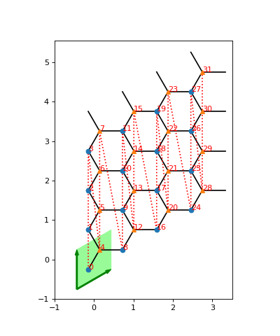
In this case, the unit cell (shaded green) consists of two sites, which for the purpose of plotting we just set to sites=None;
in general you should specify instances of Site for that.
The unit cell gets repeated in the directions given by the lattice basis (green arrows at the unit cell boundary).
Hence, we can label each site by a lattice index (x, y, u) in this case, where x in range(Lx), y in range(Ly) specify the translation of the unit cell
and u in range(len(unit_cell)), here u in [0, 1], specifies the index within the unit cell.
How an MPS winds through the lattice: the order
For MPS-based algorithms, we need to map a 2D lattice like the one above to a 1D chain.
The red, dashed line in the plot indicates how an MPS winds through the 2D
lattice. The MPS index i is a simple enumeration of the sites along this line, shown as numbers next to the sites
in the plot.
The methods mps2lat_idx() and lat2mps_idx() map
indices of the MPS to and from indices of the lattice.
The MPS class itself is (mostly) agnostic of the underlying geometry.
For example, expectation_value() will return a 1D array of the expectation value on each
site indexed by the MPS index i.
If you have a two-dimensional lattice, you can use mps2lat_values() to map this result to a 2D array index by the lattice indices.
A suitable order is critical for the efficiency of MPS-based algorithms. On one hand, different orderings can lead to different MPO bond-dimensions, with direct impact on the complexity scaling. On the other hand, it influences how much entanglement needs to go through each bonds of the underlying MPS, e.g., the ground state to be found in DMRG, and therefore influences the required MPS bond dimensions. For the latter reason, the “optimal” ordering can not be known a priori and might even depend on your coupling parameters (and the phase you are in). In the end, you can just try different orderings and see which one works best.
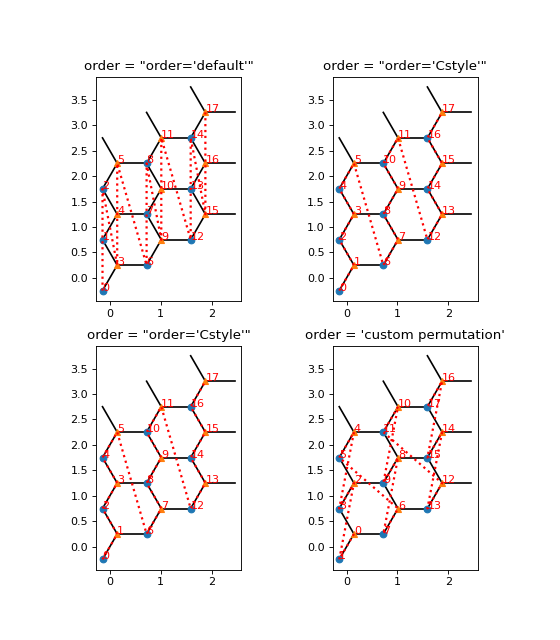
The simplest way to change the order is to use a non-default value for the initialization parameter order of the
Lattice class. This gets passed on to ordering(),
which you can override by creating a custom lattice class to define new possible orderings.
Alternatively, you can go the most general way and simply set the attribute order to be a 2D numpy array with
lattice indices as rows, in the order you want.
import matplotlib.pyplot as plt
from tenpy.models import lattice

Lx, Ly = 3, 3
fig, axes = plt.subplots(2, 2, figsize=(7, 8))

lat1 = lattice.Honeycomb(Lx, Ly, sites=None, bc='periodic')  # default order
lat2 = lattice.Honeycomb(Lx, Ly, sites=None, bc='periodic',
                        order="Cstyle")  # first method to change order
# alternative: directly set "Cstyle" order
lat3 = lattice.Honeycomb(Lx, Ly, sites=None, bc='periodic')
lat3.order = lat2.ordering("Cstyle")  # now equivalent to lat2

# general: can apply arbitrary permutation to the order
lat4 = lattice.Honeycomb(Lx, Ly, sites=None, bc='periodic',
                        order="Cstyle")
old_order = lat4.order
permutation = []
for i in range(0, len(old_order), 2):
    permutation.append(i+1)
    permutation.append(i)
lat4.order = old_order[permutation, :]

for lat, label, ax in zip([lat1, lat2, lat3, lat4],
                          ["order='default'",
                           "order='Cstyle'",
                           "order='Cstyle'",
                           "custom permutation"],
                          axes.flatten()):
    lat.plot_coupling(ax)
    lat.plot_sites(ax)
    lat.plot_order(ax, linestyle=':', linewidth=2.)
    ax.set_aspect('equal')
    ax.set_title('order = ' + repr(label))

plt.show()
(Source code, png, hires.png, pdf)

Boundary conditions
The Lattice defines the boundary conditions bc in each direction.
It can be one of the usual 'open' or 'periodic' in each direction and will be used by the
CouplingModel to determine whether there should be added periodic couplings in the
corresponding directions.
On top of that, there is the bc_MPS boundary condition of the MPS, one of 'finite', 'segment', 'infinite'.
For an 'infinite' MPS, the whole lattice is repeated in the direction of the first basis vector of the lattice.
For bc_MPS='infinite', the first direction should always be 'periodic', but you can also define a lattice with
bc_MPS='finite', bc=['periodic', 'periodic'] for a finite system on the torus.
This is discouraged, though, because the ground state MPS will require the squared bond dimension for the same precision in this
case!
For two (or higher) dimensional lattices, e.g for DMRG on an infinite cylinder,
you can also specify an integer shift instead of just saying 'periodic'.
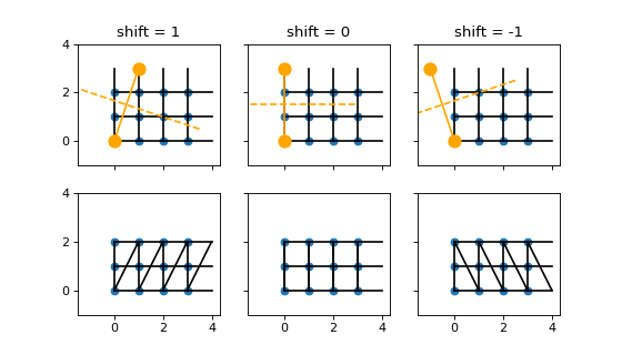
Rolling the 2D lattice up into a cylinder, you have a degree of freedom about which sites to connect.
This is illustrated in the figure below for a Square lattice with bc=['periodic', shift]
for shift in [-1, 0, 1] (different columns).
In the first row, the orange markers indicate a pair of identified sites (see plot_bc_shift()).
The dashed orange line indicates the direction of the cylinder axis.
The line where the cylinder is “cut open” therefore winds around the the cylinder for a non-zero shift.
(A similar thing happens even for shift=0 for more complicated lattices with non-orthogonal basis.)
In the second row, we directly draw lines between all sites connected by nearest-neighbor couplings, as they appear in the MPO.
(Source code, png, hires.png, pdf)

Irregular Lattices
The IrregularLattice allows you to add or remove sites from/to an existing regular lattice.
The doc-string of IrregularLattice contains several examples. Let us consider another one
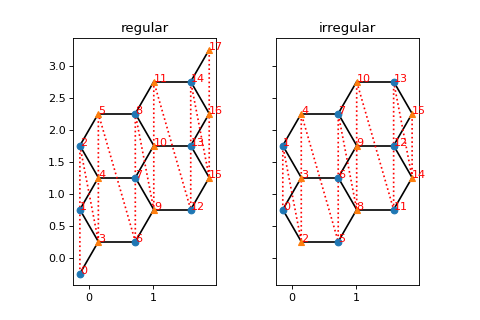
here, where we use the IrregularLattice to “fix” the boundary of the Honeycomb lattice.
When we use "open" boundary conditions for a finite system, there are two sites (shown on the lower left, and upper right corners of the figure below),
which are not included into any hexagonal. The following example shows how to remove them from the system:
import matplotlib.pyplot as plt
from tenpy.models import lattice

Lx, Ly = 3, 3
fig, axes = plt.subplots(1, 2, sharex=True, sharey=True, figsize=(6, 4))

reg_lat = lattice.Honeycomb(Lx=Lx, Ly=Ly, sites=None, bc='open')
irr_lat = lattice.IrregularLattice(reg_lat, remove=[[0, 0, 0], [-1, -1, 1]])
for lat, label, ax in zip([reg_lat, irr_lat],
                          ["regular", "irregular"],
                          axes.flatten()):
    lat.plot_coupling(ax)
    lat.plot_order(ax, linestyle=':')
    lat.plot_sites(ax)
    ax.set_aspect('equal')
    ax.set_title(label)

plt.show()
(Source code, png, hires.png, pdf)
