Overview

Repository

The root directory of the git repository contains the following folders:

tenpy

The actual source code of the library. Every subfolder contains an __init__.py file with a summary what the modules in it are good for. (This file is also necessary to mark the folder as part of the python package. Consequently, other subfolders of the git repo should not include a __init__.py file.)

toycodes

Simple toy codes completely independent of the remaining library (i.e., codes in tenpy/). These codes should be quite readable and try to give a flavor of how (some of) the algorithms work.

examples

Some example files demonstrating the usage and interface of the library, including pure python files, jupyter notebooks, and example parameter files.

doc

A folder containing the documentation: the user guide is contained in the *.rst files. The online documentation is autogenerated from these files and the docstrings of the library. This folder contains a make file for building the documentation, run make help for the different options. The necessary files for the reference in doc/reference can be auto-generated/updated with make src2html.

tests

Contains files with test routines, to be used with pytest. If you are set up correctly and have pytest installed, you can run the test suite with pytest from within the tests/ folder.

build

This folder is not distributed with the code, but is generated by setup.py (or compile.sh, respectively). It contains compiled versions of the Cython files, and can be ignored (and even removed without loosing functionality).

Layer structure

There are several layers of abstraction in TeNPy. While there is a certain hierarchy of how the concepts build up on each other, the user can decide to utilize only some of them. A maximal flexibility is provided by an object oriented style based on classes, which can be inherited and adjusted to individual demands.

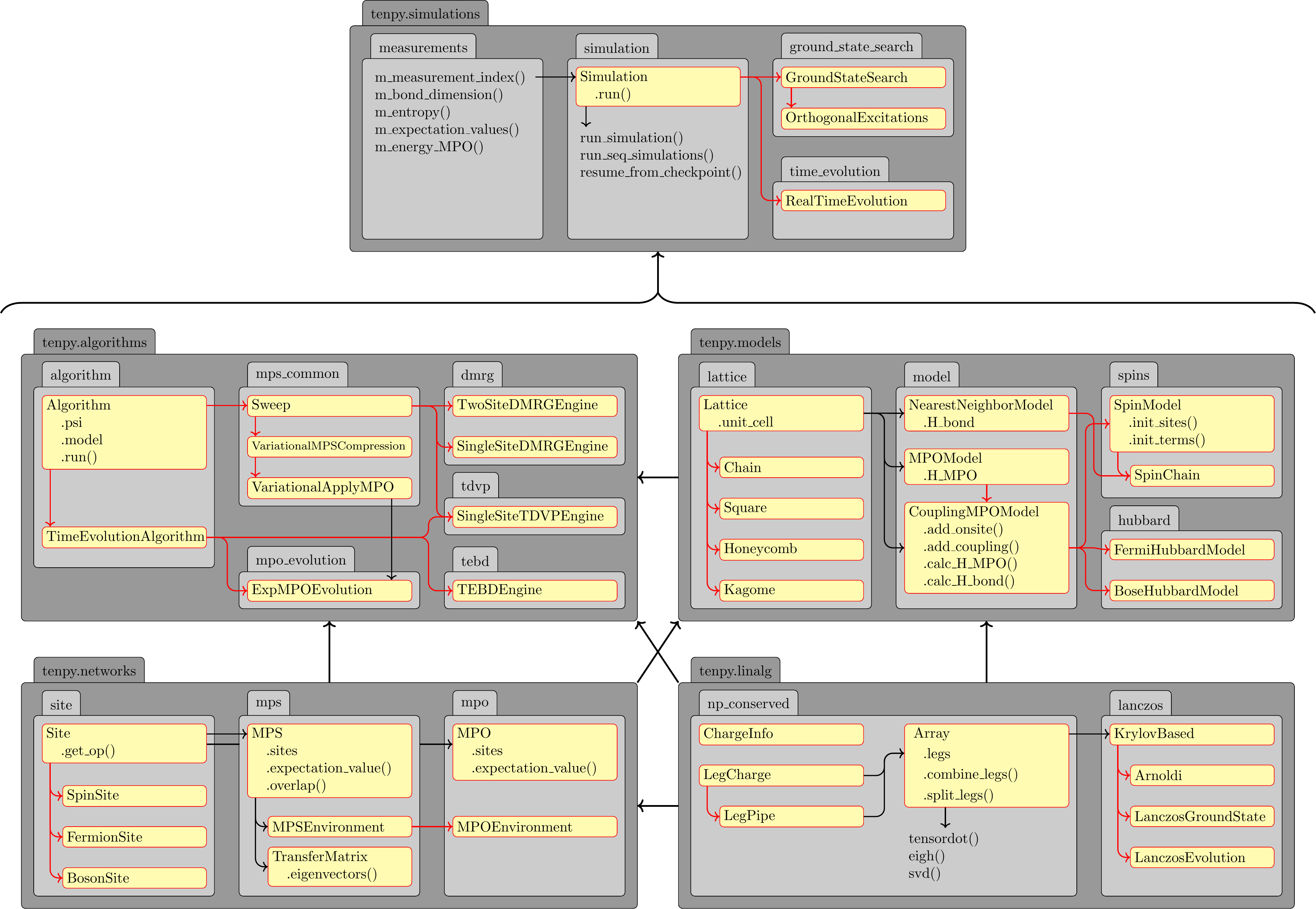
The following figure gives an overview of the most important modules, classes and functions in TeNPy. Gray backgrounds indicate (sub)modules, yellow backgrounds indicate classes. Red arrows indicate inheritance relations, dashed black arrows indicate a direct use. (The individual models might be derived from the NearestNeighborModel depending on the geometry of the lattice.) There is a fairly clear hierarchy from top-level simulations wrapping everything you want to do in a single job, over high-level algorithms in the tenpy.algorithms module down to basic operations from linear algebra in the tenpy.linalg module.

High-level simulations

The high-level interface is given by simulations, which probably handle everything you want to run on a computing cluster job: Given a set of parameters (often in the form of a parameter input file), the simulation consists of initializing the model, tensor network and algorithms, running the algorithm, performing some measurements and finally saving the results to disk. It also provides some extra functionality like the ability to resume an interrupted simulation, e.g., if your job got killed on the cluster due to runtime limits. Ideally, the simulation (sub) class represents the whole simulation from start to end, giving reproducible results depending only on the parameters given to it.

For example, calling tenpy-run parameters.yml from the terminal with the following content in the parameters.yml file will run DMRG for a SpinChain:

simulation_class: GroundStateSearch

output_filename: results.h5

model_class:  SpinChain
model_params:
    L: 32
    bc_MPS: finite
    Jz: 1.

initial_state_params:
    method: lat_product_state
    product_state: [[up], [down]]

algorithm_class: TwoSiteDMRGEngine
algorithm_params:
    trunc_params:
        svd_min: 1.e-10
        chi_max: 100
    mixer: True

Note

The Simulations user guide is a good point to continue reading when you finished reading this overview.

To get a sense how things work together, it’s instructive to consider the remaining layers in a bottom-to-top order.

Low-level: tensors and linear algebra

Note

See Charge conservation with np_conserved for more information on defining charges for arrays.

The most basic layer is given by in the linalg module, which provides basic features of linear algebra. In particular, the np_conserved submodule implements an Array class which is used to represent the tensors. The basic interface of np_conserved is very similar to that of the NumPy and SciPy libraries. However, the Array class implements abelian charge conservation. If no charges are to be used, one can use ‘trivial’ arrays, as shown in the following example code.

"""Basic use of the `Array` class with trivial arrays."""

import tenpy.linalg.np_conserved as npc

M = npc.Array.from_ndarray_trivial([[0., 1.], [1., 0.]])
v = npc.Array.from_ndarray_trivial([2., 4. + 1.j])
v[0] = 3.  # set indiviual entries like in numpy
print("|v> =", v.to_ndarray())
# |v> = [ 3.+0.j  4.+1.j]

M_v = npc.tensordot(M, v, axes=[1, 0])
print("M|v> =", M_v.to_ndarray())
# M|v> = [ 4.+1.j  3.+0.j]
print("<v|M|v> =", npc.inner(v.conj(), M_v, axes='range'))
# <v|M|v> = (24+0j)

The number and types of symmetries are specified in a ChargeInfo class. An Array instance represents a tensor satisfying a charge rule specifying which blocks of it are nonzero. Internally, it stores only the non-zero blocks of the tensor, along with one LegCharge instance for each leg, which contains the charges and sign qconj for each leg. We can combine multiple legs into a single larger LegPipe, which is derived from the LegCharge and stores all the information necessary to later split the pipe.

The following code explicitly defines the spin-1/2 \(S^+, S^-, S^z\) operators and uses them to generate and diagonalize the two-site Hamiltonian \(H = \vec{S} \cdot \vec{S}\). It prints the charge values (by default sorted ascending) and the eigenvalues of H.

"""Explicit definition of charges and spin-1/2 operators."""

import tenpy.linalg.np_conserved as npc

# consider spin-1/2 with Sz-conservation
chinfo = npc.ChargeInfo([1])  # just a U(1) charge
# charges for up, down state
p_leg = npc.LegCharge.from_qflat(chinfo, [[1], [-1]])
Sz = npc.Array.from_ndarray([[0.5, 0.], [0., -0.5]], [p_leg, p_leg.conj()])
Sp = npc.Array.from_ndarray([[0., 1.], [0., 0.]], [p_leg, p_leg.conj()])
Sm = npc.Array.from_ndarray([[0., 0.], [1., 0.]], [p_leg, p_leg.conj()])

Hxy = 0.5 * (npc.outer(Sp, Sm) + npc.outer(Sm, Sp))
Hz = npc.outer(Sz, Sz)
H = Hxy + Hz
# here, H has 4 legs
H.iset_leg_labels(["s1", "t1", "s2", "t2"])
H = H.combine_legs([["s1", "s2"], ["t1", "t2"]], qconj=[+1, -1])
# here, H has 2 legs
print(H.legs[0].to_qflat().flatten())
# prints [-2  0  0  2]
E, U = npc.eigh(H)  # diagonalize blocks individually
print(E)
# [ 0.25 -0.75  0.25  0.25]

Sites for the local Hilbert space and tensor networks

The next basic concept is that of a local Hilbert space, which is represented by a Site in TeNPy. This class does not only label the local states and define the charges, but also provides onsite operators. For example, the SpinHalfSite provides the \(S^+, S^-, S^z\) operators under the names 'Sp', 'Sm', 'Sz', defined as Array instances similarly as in the code above. Since the most common sites like for example the SpinSite (for general spin S=0.5, 1, 1.5,…), BosonSite and FermionSite are predefined, a user of TeNPy usually does not need to define the local charges and operators explicitly. The total Hilbert space, i.e, the tensor product of the local Hilbert spaces, is then just given by a list of Site instances. If desired, different kinds of Site can be combined in that list. This list is then given to classes representing tensor networks like the MPS and MPO. The tensor network classes also use Array instances for the tensors of the represented network.

The following example illustrates the initialization of a spin-1/2 site, an MPS representing the Neel state, and an MPO representing the Heisenberg model by explicitly defining the W tensor.

"""Initialization of sites, MPS and MPO."""

from tenpy.networks.site import SpinHalfSite
from tenpy.networks.mps import MPS
from tenpy.networks.mpo import MPO

spin = SpinHalfSite(conserve="Sz")

N = 6  # number of sites
sites = [spin] * N  # repeat entry of list N times
pstate = ["up", "down"] * (N // 2)  # Neel state
psi = MPS.from_product_state(sites, pstate, bc="finite")
print("<Sz> =", psi.expectation_value("Sz"))
# <Sz> = [ 0.5 -0.5  0.5 -0.5]
print("<Sp_i Sm_j> =", psi.correlation_function("Sp", "Sm"), sep="\n")
# <Sp_i Sm_j> =
# [[1. 0. 0. 0. 0. 0.]
#  [0. 0. 0. 0. 0. 0.]
#  [0. 0. 1. 0. 0. 0.]
#  [0. 0. 0. 0. 0. 0.]
#  [0. 0. 0. 0. 1. 0.]
#  [0. 0. 0. 0. 0. 0.]]

# define an MPO
Id, Sp, Sm, Sz = spin.Id, spin.Sp, spin.Sm, spin.Sz
J, Delta, hz = 1., 1., 0.2
W_bulk = [[Id, Sp, Sm, Sz, -hz * Sz], [None, None, None, None, 0.5 * J * Sm],
          [None, None, None, None, 0.5 * J * Sp], [None, None, None, None, J * Delta * Sz],
          [None, None, None, None, Id]]
W_first = [W_bulk[0]]  # first row
W_last = [[row[-1]] for row in W_bulk]  # last column
Ws = [W_first] + [W_bulk] * (N - 2) + [W_last]
H = MPO.from_grids([spin] * N, Ws, bc='finite', IdL=0, IdR=-1)
print("<psi|H|psi> =", H.expectation_value(psi))
# <psi|H|psi> = -1.25

Models

Note

See Models for more information on sites and how to define and extend models on your own.

Technically, the explicit definition of an MPO is already enough to call an algorithm like DMRG in dmrg. However, writing down the W tensors is cumbersome especially for more complicated models. Hence, TeNPy provides another layer of abstraction for the definition of models, which we discuss first. Different kinds of algorithms require different representations of the Hamiltonian. Therefore, the library offers to specify the model abstractly by the individual onsite terms and coupling terms of the Hamiltonian. The following example illustrates this, again for the Heisenberg model.

"""Definition of a model: the XXZ chain."""

from tenpy.networks.site import SpinSite
from tenpy.models.lattice import Chain
from tenpy.models.model import CouplingModel, NearestNeighborModel, MPOModel


class XXZChain(CouplingModel, NearestNeighborModel, MPOModel):
    def __init__(self, L=2, S=0.5, J=1., Delta=1., hz=0.):
        spin = SpinSite(S=S, conserve="Sz")
        # the lattice defines the geometry
        lattice = Chain(L, spin, bc="open", bc_MPS="finite")
        CouplingModel.__init__(self, lattice)
        # add terms of the Hamiltonian
        self.add_coupling(J * 0.5, 0, "Sp", 0, "Sm", 1)  # Sp_i Sm_{i+1}
        self.add_coupling(J * 0.5, 0, "Sp", 0, "Sm", -1)  # Sp_i Sm_{i-1}
        self.add_coupling(J * Delta, 0, "Sz", 0, "Sz", 1)
        # (for site dependent prefactors, the strength can be an array)
        self.add_onsite(-hz, 0, "Sz")

        # finish initialization
        # generate MPO for DMRG
        MPOModel.__init__(self, lattice, self.calc_H_MPO())
        # generate H_bond for TEBD
        NearestNeighborModel.__init__(self, lattice, self.calc_H_bond())

While this generates the same MPO as in the previous code, this example can easily be adjusted and generalized, for example to a higher dimensional lattice by just specifying a different lattice. Internally, the MPO is generated using a finite state machine picture. This allows not only to translate more complicated Hamiltonians into their corresponding MPOs, but also to automate the mapping from a higher dimensional lattice to the 1D chain along which the MPS winds. Note that this mapping introduces longer-range couplings, so the model can no longer be defined to be a NearestNeighborModel suited for TEBD if another lattice than the Chain is to be used. Of course, many commonly studied models are also predefined. For example, the following code initializes the Heisenberg model on a kagome lattice; the spin liquid nature of the ground state of this model is highly debated in the current literature.

"""Initialization of the Heisenberg model on a kagome lattice."""

from tenpy.models.spins import SpinModel

model_params = {
    "S": 0.5,  # Spin 1/2
    "lattice": "Kagome",
    "bc_MPS": "infinite",
    "bc_y": "cylinder",
    "Ly": 2,  # defines cylinder circumference
    "conserve": "Sz",  # use Sz conservation
    "Jx": 1.,
    "Jy": 1.,
    "Jz": 1.  # Heisenberg coupling
}
model = SpinModel(model_params)

Algorithms

The highest level beyond the wrapping simulations) is given by algorithms like DMRG and TEBD. They usually need to be initialized with a state, i.e., tensor network like an MPS, and suitable model. Those are defined in the next lower levels. The following simple example illustrates the basic structure that the simulation class needs to perform for the same parameters as the example above, calling the cl:mod:~tenpy.algorithms.dmrg.

"""Call of (finite) DMRG."""

from tenpy.networks.mps import MPS
from tenpy.models.tf_ising import TFIChain
from tenpy.algorithms import dmrg

N = 16  # number of sites
model = TFIChain({"L": N, "J": 1., "g": 1., "bc_MPS": "finite"})
sites = model.lat.mps_sites()
psi = MPS.from_product_state(sites, ['up'] * N, "finite")
dmrg_params = {"trunc_params": {"chi_max": 100, "svd_min": 1.e-10}, "mixer": True}
info = dmrg.run(psi, model, dmrg_params)
print("E =", info['E'])
# E = -20.01638790048513
print("max. bond dimension =", max(psi.chi))
# max. bond dimension = 27

The switch from DMRG to iDMRG in TeNPy is simply accomplished by a change of the parameter "bc_MPS" from "finite" to "infinite", both for the model and the state. The returned E is then the energy density per site. Due to the translation invariance, one can also evaluate the correlation length, here slightly away from the critical point.

"""Call of infinite DMRG."""

from tenpy.networks.mps import MPS
from tenpy.models.tf_ising import TFIChain
from tenpy.algorithms import dmrg

N = 2  # number of sites in unit cell
model = TFIChain({"L": N, "J": 1., "g": 1.1, "bc_MPS": "infinite"})
sites = model.lat.mps_sites()
psi = MPS.from_product_state(sites, ['up'] * N, "infinite")
dmrg_params = {"trunc_params": {"chi_max": 100, "svd_min": 1.e-10}, "mixer": True}
info = dmrg.run(psi, model, dmrg_params)
print("E =", info['E'])
# E = -1.342864022725017
print("max. bond dimension =", max(psi.chi))
# max. bond dimension = 56
print("corr. length =", psi.correlation_length())
# corr. length = 4.915809146764157

Running time evolution with TEBD requires an additional loop, during which the desired observables have to be measured. The following code shows this directly for the infinite version of TEBD.

"""Call of (infinite) TEBD."""

from tenpy.networks.mps import MPS
from tenpy.models.tf_ising import TFIChain
from tenpy.algorithms import tebd

M = TFIChain({"L": 2, "J": 1., "g": 1.5, "bc_MPS": "infinite"})
psi = MPS.from_product_state(M.lat.mps_sites(), [0] * 2, "infinite")
tebd_params = {
    "order": 2,
    "delta_tau_list": [0.1, 0.001, 1.e-5],
    "max_error_E": 1.e-6,
    "trunc_params": {
        "chi_max": 30,
        "svd_min": 1.e-10
    }
}
eng = tebd.TEBDEngine(psi, M, tebd_params)
eng.run_GS()  # imaginary time evolution with TEBD
print("E =", sum(psi.expectation_value(M.H_bond)) / psi.L)
print("final bond dimensions: ", psi.chi)

Note that there is also a simulation class for RealTimeEvolution that can handle this extra loop over time, and allows to easily switch between different time evolution algorithms.