purification_mps
full name: tenpy.networks.purification_mps
parent module:
tenpy.networkstype: module
Classes
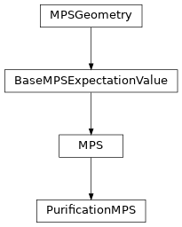
|
An MPS representing a finite-temperature ensemble using purification. |
Functions
|
Extend charges of model for |
Module description
This module contains an MPS class representing an density matrix by purification.
Usually, an MPS represents a pure state, i.e. the density matrix is \(\rho = |\psi><\psi|\), describing observables as \(<O> = Tr(O|\psi><\psi|) = <\psi|O|\psi>\). Clearly, if \(|\psi>\) is the ground state of a Hamiltonian, this is the density matrix at T=0.
At finite temperatures \(T > 0\), we want to describe a mixed density matrix \(\rho = \exp(-H/T)\). The following approaches have been used to lift the power of tensor network ansätze (representing pure states= to finite temperatures (and mixed states in general).
Naively represent the density matrix as an MPO. This has the disadvantage that truncation can quickly lead to non-positive (and hence unphysical) density matrices.
Minimally entangled typical thermal states (METTS) as introduced in [white2009].
Use Purification to represent the mixed density matrix by pure states in the doubled Hilbert space. In the literature, this is also referred to as matrix product density operators (MPDO) or locally purified density operator (LPDO).
Here, we follow the third approach. In addition to the physical space P, we introduce a second ‘auxiliary’ space Q and define the density matrix of the physical system as \(\rho = Tr_Q(|\phi><\phi|)\), where \(|\phi>\) is a pure state in the combined physical and auxiliary system.
For \(T=\infty\), the density matrix \(\rho_\infty\) is the identity matrix.
In other words, expectation values are sums over all possible states
\(<O> = Tr_P(\rho_\infty O) = Tr_P(O)\).
Saying that each : on top is to be connected with the corresponding : on the bottom,
the trace is simply a contraction:
|         :   :   :   :   :   :
|         |   |   |   |   |   |
|         |-------------------|
|         |        O          |
|         |-------------------|
|         |   |   |   |   |   |
|         :   :   :   :   :   :
Clearly, we get the same result, if we insert an identity operator, written as MPO, on the top and bottom:
|         :   :   :   :   :   :
|         |   |   |   |   |   |
|         B---B---B---B---B---B
|         |   |   |   |   |   |
|         |-------------------|
|         |        O          |
|         |-------------------|
|         |   |   |   |   |   |
|         B*--B*--B*--B*--B*--B*
|         |   |   |   |   |   |
|         :   :   :   :   :   :
We use the following label convention:
|         q
|         ^
|         |
|  vL ->- B ->- vR
|         |
|         ^
|         p
You can view the MPO as an MPS by combining the p and q leg and defining every physical operator to act trivial on the q leg. In expectation values, you would then sum over over the q legs, which is exactly what we need. In other words, the choice \(B = \delta_{p,q}\) with trivial (length-1) virtual bonds yields infinite temperature expectation values for operators action only on the p legs!
Now, you go a step further and also apply imaginary time evolution (acting only on p legs) to the initial infinite temperature state. For example, the normalized state \(|\psi> \propto \exp(-\beta/2 H)|\phi>\) yields expectation values
An additional real-time evolution allows to calculate time correlation functions:
Time evolution algorithms (TEBD and MPO application) are adjusted in the module
purification.
See also [karrasch2013] for additional tricks! One of their crucial observations is, that
one can apply arbitrary unitaries on the auxiliary space (i.e. the q) without changing the result.
This can actually be used to reduce the necessary virtual bond dimensions:
From the definition, it is easy to see that if we apply \(exp(-i H t)\) to the p legs of
\(|\phi>\), and \(\exp(+iHt)\) to the q legs, they just cancel out!
(They commute with \(\exp(-\beta H/2)\)…)
If the state is modified (e.g. by applying A or B to calculate correlation functions),
this is not true any more. However, we still can find unitaries, which are ‘optimal’ in the sense
of reducing the entanglement of the MPS/MPO to the minimal value.
For a discussion of Disentanglers (implemented in disentanglers),
see [hauschild2018].
Note
The classes MPSEnvironment and
TransferMatrix should also work for the
PurificationMPS defined here.
For example, you can use expectation_value()
for the expectation value of operators between different PurificationMPS.
However, this makes only sense if the same disentangler was applied
to the bra and ket PurificationMPS.
Note
The literature (e.g. section 7.2 of [schollwoeck2011] or [karrasch2013]) suggests to use a singlet as a maximally entangled state. Here, we use instead the identity \(\delta_{p,q}\), since it is easier to generalize for p running over more than two indices, and allows a simple use of charge conservation with the above qconj convention. Moreover, we don’t split the physical and auxiliary space into separate sites, which makes TEBD as costly as \(O(d^6 \chi^3)\).