MPS
full name: tenpy.networks.mps.MPS
parent module:
tenpy.networks.mpstype: class
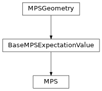
Inheritance Diagram
Methods
|
|
|
Return an MPS which represents |
|
Apply signs on a virtual MPS leg equivalent to a Jordan-Wigner string on the left. |
|
Apply a local (one or multi-site) operator to self. |
|
Similar as |
|
Apply a (global) product of local onsite operators to self. |
|
Return the average charge for the block on the left of a given bond. |
|
Bring self into canonical 'B' form, (re-)calculate singular values; in place. |
|
Bring a finite (or segment) MPS into canonical form; in place. |
|
Bring an infinite MPS into canonical form; in place. |
|
Convert infinite MPS to canonical form; in place. |
|
Return the charge variance on the left of a given bond. |
|
Compress an MPS. |
|
Compress self with a single sweep of SVDs; in place. |
|
Compute the momentum quantum numbers of the entanglement spectrum for 2D states. |
|
Transform self into different canonical form (by scaling the legs with singular values). |
|
Returns a copy of self. |
|
Correlation function of single-site operators. |
|
Calculate the correlation length by diagonalizing the transfer matrix. |
|
Calculate the correlation length by diagonalizing the transfer matrix. |
Return possible charge_sector argument for |
|
|
Artificially enlarge the bond dimension by the specified extra legs/charges. |
|
Repeat the unit cell for infinite MPS boundary conditions; in place. |
|
Calculate the (half-chain) entanglement entropy for all nontrivial bonds. |
|
Calculate entanglement entropy for general geometry of the bipartition. |
|
Calculate entanglement entropy for general geometry of the bipartition. |
|
Return entanglement energy spectrum. |
|
Expectation value |
|
Expectation value |
|
Expectation value |
|
Calculate expectation values for a bunch of terms and sum them up. |
|
Extract an enlarged segment from an initially smaller segment MPS. |
|
Extract an segment from a finite or infinite MPS. |
|
Construct a matrix product state from a set of numpy arrays Bflat and singular vals. |
|
Construct a matrix product state with given bond dimensions from random matrices. |
|
Construct an MPS from a single tensor psi with one leg per physical site. |
|
Load instance from a HDF5 file. |
|
Construct an MPS from a product state given in lattice coordinates. |
|
Create an MPS as a product of (many) local mps covering all sites to be created. |
|
Construct a matrix product state from a given product state. |
|
Construct a matrix product state by evolving a product state with random unitaries. |
|
Create an MPS of entangled singlets. |
|
Gauge the legcharges of the virtual bonds s.t. |
|
Return (view of) B at site i in canonical form. |
|
Return singular values on the left of site i. |
|
Return singular values on the right of site i. |
Construct the charge-tree for a given charge sector. |
|
|
Like |
|
Given a list of operators, select the one corresponding to site i. |
|
Return reduced density matrix for a segment. |
|
Get the i-th site. |
|
Calculates the n-site wavefunction on |
|
Calculate and return the qtotal of the whole MPS (when contracted). |
|
Modify self inplace to group sites. |
|
Modify self inplace to split previously grouped sites. |
|
Calculate the two-site mutual information \(I(i:j)\). |
Check that self is in canonical form. |
|
Return the virtual legs on the left and right of the MPS. |
|
|
Compute overlap |
|
Contract |
|
Applies the permutation perm to the state; in place. |
|
Locally perturb the state a little bit; in place. |
|
Return probabilities of charge value on the left of a given bond. |
|
Generates an MPS from a product state list which is projected onto a given charge sector. |
|
Shift the section we define as unit cell of an infinite MPS; in place. |
|
Sample measurement results in the computational basis. |
|
Export self into a HDF5 file. |
|
Set B at site i. |
|
Set singular values on the left of site i. |
|
Set singular values on the right of site i. |
|
SVD a two-site wave function theta and save it in self. |
|
Shift an Array by an integer multiple of unit cells. |
|
Shift a site by an integer multiple of unit cells. |
|
Shift charges by an integer multiple of unit cells. |
Perform a spatial inversion along the MPS. |
|
|
Subspace expansion increasing chi without changing the represented state. |
|
Swap the two neighboring sites i and i+1; in place. |
|
Correlation function between (multi-site) terms, moving the left term, fix right term. |
|
Correlation function between (multi-site) terms, moving the right term, fix left term. |
Correlation function between sums of multi-site terms, moving the right sum of term. |
|
Sanity check, raises ValueErrors, if something is wrong. |
Class Attributes and Properties
Number of physical sites; for an iMPS the len of the MPS unit cell. |
|
Number of sites per horizontal lattice spacing. |
|
Dimensions of the (nontrivial) virtual bonds. |
|
List of local physical dimensions. |
|
Distinguish MPS vs iMPS. |
|
Slice of the non-trivial bond indices, depending on |
- class tenpy.networks.mps.MPS(sites, Bs, SVs, bc='finite', form='B', norm=1.0, unit_cell_width=None, understood_shift_symmetry: bool = False)[source]
Bases:
BaseMPSExpectationValueA Matrix Product State, finite (MPS) or infinite (iMPS).
- Parameters:
sites (list of
Site) – Defines the local Hilbert space for each site.Bs (list of
Array) – The ‘matrices’ of the MPS. Labels arevL, vR, p(in any order).SVs (list of 1D array) – The singular values on each bond. Should always have length L+1. Entries out of
nontrivial_bondsare ignored.form ((list of) {
'B' | 'A' | 'C' | 'G' | 'Th' | None| tuple(float, float)}) – The form of the stored ‘matrices’, see table in module doc-string. A single choice holds for all of the entries.
- form
Describes the canonical form on each site.
Nonemeans non-canonical form. Forform = (nuL, nuR), the stored_B[i]ares**form[0] -- Gamma -- s**form[1](in Vidal’s notation).- Type:
list of {
None, tuple(float, float)}
- norm
The overall norm of the state, i.e.
sqrt(<psi|psi>)- the tensors are kept normalized. Ignored for (normalized)expectation_value()and co, but important foroverlap()and expectation value methods ofMPSEnvironment.- Type:
- grouped
Number of sites grouped together, see
group_sites().- Type:
- segment_boundaries
Only defined for ‘segment’ bc if
canonical_form_finite()has been called. If defined, it contains the U_L and V_R that would be returned by that function.- Type:
tuple of
Array| (None, None)
- _B
The ‘matrices’ of the MPS. Labels are
vL, vR, p(in any order). We recommend usingget_B()andset_B(), which will take care of the different canonical forms.- Type:
list of
npc.Array
- _S
The singular values on each virtual bond, length
L+1. May beNoneif the MPS is not in canonical form. Otherwise,_S[i]is to the left of_B[i]. We recommend usingget_SL(),get_SR(),set_SL(),set_SR(), which takes proper care of the boundary conditions. Sometimes (e.g. during DMRG with an enabled mixer), entries may temporarily be a non-diagonaltenpy.linalg.np_conserved.Arrayto be inserted between the left canonical ‘A’ tensors on the left and right-canonical _B[i] on the right.- Type:
list of {
None, 1D array,Array}
- _valid_forms
Class attribute. Mapping for canonical forms to a tuple
(nuL, nuR)indicating thatself._B[i] = s[i]**nuL -- Gamma[i] -- s[i]**nuRis saved.- Type:
- _transfermatrix_keep
How many states to keep at least when diagonalizing a
TransferMatrix. Important if the state develops a near-degeneracy.- Type:
- _p_label, _B_labels
Class attribute. _p_label defines the physical legs of the B-tensors, _B_labels lists all the labels of the B tensors. Used by methods like
get_theta()to avoid the necessity of re-implementations for derived classes like thePurification_MPSif just the number of physical legs changed.
- copy()[source]
Returns a copy of self.
The copy still shares the sites, chinfo, and LegCharges of the B tensors, but the values of B and S are deeply copied.
- save_hdf5(hdf5_saver, h5gr, subpath)[source]
Export self into a HDF5 file.
This method saves all the data it needs to reconstruct self with
from_hdf5().Specifically, it saves
sites,chinfo,unit_cell_width(under these names),_Bas"tensors",_Sas"singular_values",bcas"boundary_condition",formconverted to a single array of shape (L, 2) as"canonical_form". Moreover, it savesnorm,L,groupedand_transfermatrix_keep(as “transfermatrix_keep”) as HDF5 attributes, as well as the maximum ofchiunder the name “max_bond_dimension”.
- classmethod from_hdf5(hdf5_loader, h5gr, subpath)[source]
Load instance from a HDF5 file.
This method reconstructs a class instance from the data saved with
save_hdf5().- Parameters:
hdf5_loader (
Hdf5Loader) – Instance of the loading engine.h5gr (
Group) – HDF5 group which is represent the object to be constructed.subpath (str) – The name of h5gr with a
'/'in the end.
- Returns:
obj – Newly generated class instance containing the required data.
- Return type:
cls
- classmethod from_lat_product_state(lat, p_state, allow_incommensurate=False, **kwargs)[source]
Construct an MPS from a product state given in lattice coordinates.
This is a wrapper around
from_product_state(). The purpose is to make the p_state argument independent of the order of the Lattice, and specify it in terms of lattice indices instead.- Parameters:
lat (
Lattice) – The underlying lattice defining the geometry and Hilbert Space.p_state (array_like of {int | str | 1D array}) – Defines the product state to be represented. Should be of dimension lat.dim`+1, entries are indexed by lattice indices. Entries of the array as for the `p_state argument of
from_product_state(). It gets tiled to the shapelat.shape, if it is smaller.allow_incommensurate (bool) – Allow an incommensurate tiling of p_state to the full lattice. For example, if you pass
p_state=[['up'], ['down']]with atenpy.models.lattice.Chain, this function raises an error for an odd number of sites in the Chain, but if you set allow_incommensurate=True, it will still work and give you a state with total Sz = +1/2 for odd sites (since total Sz=0 doesn’t fit).**kwargs – Other keyword arguments as defined in
from_product_state(). bc is set by default fromlat.bc_MPS.
- Returns:
product_mps – An MPS representing the specified product state.
- Return type:
Examples
Let’s first consider a
Laddercomposed of aSpinHalfSiteand aFermionSite.To initialize a state of up-spins on the spin sites and half-filled fermions, you can use:
Note that the same p_state works for a finite lattice of even length, say
L=10, as well. We then just “tile” in x-direction, i.e., repeat the specified state 5 times:You can also easily half-fill a
Honeycomb, for example with only the A sites occupied, or as stripe parallel to the x-direction (stripe_x, alternating along y axis), or as stripes parallel to the y-direction (stripe_y, alternating along x axis).
- classmethod from_product_state(sites, p_state, bc='finite', dtype=<class 'numpy.float64'>, permute=True, form='B', chargeL=None, unit_cell_width=None, understood_shift_symmetry: bool = False)[source]
Construct a matrix product state from a given product state.
- Parameters:
sites (list of
Site) – The sites defining the local Hilbert space.p_state (list of {int | str | 1D array}) – Defines the product state to be represented; one entry for each site of the MPS. An entry of str type is translated to an int with the help of
state_labels(). An entry of int type represents the physical index of the state to be used. An entry which is a 1D array defines the complete wavefunction on that site; this allows to make a (local) superposition.bc ({'infinite', 'finite', 'segment'}) – MPS boundary conditions. See docstring of
MPS.dtype (type or string) – The data type of the array entries.
permute (bool) – The
Sitemight permute the local basis states if charge conservation gets enabled. If permute is True (default), we permute the given p_state locally according to each site’sperm. The p_state entries should then always be given as if conserve=None in the Site.form ((list of) {
'B' | 'A' | 'C' | 'G' | None| tuple(float, float)}) – Defines the canonical form. See module doc-string. A single choice holds for all of the entries.chargeL (charges) – Leg charges at bond 0, which are purely conventional.
unit_cell_width (int) – See
mps_unit_cell_width.
- Returns:
product_mps – An MPS representing the specified product state.
- Return type:
Examples
Example to get a Neel state for a
TFIChain:>>> from tenpy.networks.mps import MPS >>> L = 10 >>> M = tenpy.models.tf_ising.TFIChain({'L': L}) >>> p_state = ['up', 'down'] * (L // 2) # repeats entries L/2 times >>> psi = MPS.from_product_state( ... M.lat.mps_sites(), p_state, bc=M.lat.bc_MPS, unit_cell_width=M.lat.mps_unit_cell_width ... )
The meaning of the labels
"up","down"is defined by theSite, in this example aSpinHalfSite.Extending the example, we can replace the spin in the center with one with arbitrary angles
theta, phiin the bloch sphere. However, note that you can not write this bloch state (fortheta != 0, pi) when conserving symmetries, as the two physical basis states correspond to different symmetry sectors.>>> spin = tenpy.networks.site.SpinHalfSite(conserve=None, sort_charge=False) >>> p_state = ['up', 'down'] * (L // 2) # repeats entries L/2 times >>> theta, phi = np.pi / 4, np.pi / 6 >>> bloch_sphere_state = np.array([np.cos(theta / 2), np.exp(1.0j * phi) * np.sin(theta / 2)]) >>> p_state[L // 2] = bloch_sphere_state # replace one spin in center >>> psi = MPS.from_product_state( ... [spin] * L, p_state, bc=M.lat.bc_MPS, dtype=complex, unit_cell_width=M.lat.mps_unit_cell_width ... )
Note that for the more general
SpinChain, the order of the two entries for thebloch_sphere_statewould be exactly the opposite (when we keep the the north-pole of the bloch sphere being the up-state). The reason is that the SpinChain uses the generalSpinSite, where the states are ordered ascending from'down'to'up'. TheSpinHalfSiteon the other hand uses the order'up', 'down'where that the Pauli matrices look as usual.
- classmethod from_random_unitary_evolution(sites, chi, p_state, bc='finite', dtype=<class 'numpy.float64'>, permute=True, form='B', chargeL=None, understood_shift_symmetry: bool = False)[source]
Construct a matrix product state by evolving a product state with random unitaries.
- Parameters:
sites (list of
Site) – The sites defining the local Hilbert space.chi (int) – The target bond dimension. For finite systems, we evolve until the maximum bond dimension reaches this value. For infinite systems, we evolve until all bond dimensions have reached this value.
p_state (list of {int | str | 1D array}) – Defines the product state to start from; one entry for each site of the MPS. An entry of str type is translated to an int with the help of
state_labels(). An entry of int type represents the physical index of the state to be used. An entry which is a 1D array defines the complete wavefunction on that site; this allows to make a (local) superposition.bc ({'infinite', 'finite', 'segment'}) – MPS boundary conditions. See docstring of
MPS.dtype (type or string) – The data type of the array entries.
permute (bool) – The
Sitemight permute the local basis states if charge conservation gets enabled. If permute is True (default), we permute the given p_state locally according to each site’sperm. The p_state entries should then always be given as if conserve=None in the Site.form ((list of) {
'B' | 'A' | 'C' | 'G' | None| tuple(float, float)}) – Defines the canonical form. See module doc-string. A single choice holds for all of the entries.chargeL (charges) – Leg charges at bond 0, which are purely conventional.
- classmethod from_desired_bond_dimension(sites, chis, bc='finite', dtype=<class 'numpy.float64'>, permute=True, chargeL=None, unit_cell_width=None, understood_shift_symmetry: bool = False)[source]
Construct a matrix product state with given bond dimensions from random matrices.
Note: no charge conservation
- Parameters:
sites (list of
Site) – The sites defining the local Hilbert space.chis ((list of) {int}) – Desired bond dimensions. For a single int, the same bond dimension is used on every bond.
bc ({'infinite', 'finite'}) – MPS boundary conditions. See docstring of
MPS. For ‘finite’ chi is capped to the maximum possible at each bond.dtype (type or string) – The data type of the array entries.
permute (bool) – The
Sitemight permute the local basis states if charge conservation gets enabled. If permute is True (default), we permute the given p_state locally according to each site’sperm. The p_state entries should then always be given as if conserve=None in the Site.chargeL (charges) – Leg charges at bond 0, which are purely conventional.
unit_cell_width (int) – See
mps_unit_cell_width.
- Returns:
mps – An MPS with the desired bond dimension.
- Return type:
- classmethod from_Bflat(sites, Bflat, SVs=None, bc='finite', dtype=None, permute=True, form='B', legL=None, unit_cell_width=None, understood_shift_symmetry: bool = False)[source]
Construct a matrix product state from a set of numpy arrays Bflat and singular vals.
- Parameters:
sites (list of
Site) – The sites defining the local Hilbert space.Bflat (iterable of numpy ndarrays) – The matrix defining the MPS on each site, with legs
'p', 'vL', 'vR'(physical, virtual left/right).SVs (list of 1D array |
None) – The singular values on each bond. Should always have length L+1. By default (None), set all singular values to the same value. Entries out ofnontrivial_bondsare ignored.bc ({'infinite', 'finite', 'segment'}) – MPS boundary conditions. See docstring of
MPS.dtype (type or string) – The data type of the array entries. Defaults to the common dtype of Bflat.
permute (bool) – The
Sitemight permute the local basis states if charge conservation gets enabled. If permute is True (default), we permute the given Bflat locally according to each site’sperm. The Bflat should then always be given as if conserve=None in the Site.form ((list of) {
'B' | 'A' | 'C' | 'G' | None| tuple(float, float)}) – Defines the canonical form of Bflat. See module doc-string. A single choice holds for all of the entries.leg_L (LegCharge |
None) – Leg charges at bond 0, which are purely conventional. IfNone, use trivial charges.unit_cell_width (int) – See
mps_unit_cell_width.
- Returns:
mps – An MPS with the matrices Bflat converted to npc arrays.
- Return type:
- classmethod from_full(sites, psi, form=None, cutoff=1e-16, normalize=True, bc='finite', outer_S=None, unit_cell_width=None, understood_shift_symmetry: bool = False)[source]
Construct an MPS from a single tensor psi with one leg per physical site.
Performs a sequence of SVDs of psi to split off the B matrices and obtain the singular values, the result will be in canonical form. Obviously, this is only well-defined for finite or segment boundary conditions.
- Parameters:
sites (list of
Site) – The sites defining the local Hilbert space.psi (
Array) – The full wave function to be represented as an MPS. Should have labels'p0', 'p1', ..., 'p{L-1}'(in any order). Additionally, it may have (or must have for ‘segment’ bc) the legs'vL', 'vR', which are trivial for ‘finite’ bc. For subclasses with multiple physical legs per site, we instead expect one set of labels per site (e.g.'p0', 'q0', 'p1', 'q1', ...forPurificationMPS).form (
'B' | 'A' | 'C' | 'G' | None) – The canonical form of the resulting MPS, see module doc-string.Nonedefaults to ‘A’ form on the first site and ‘B’ form on all following sites.cutoff (float) – Cutoff of singular values used in the SVDs.
normalize (bool) – Whether the resulting MPS should have ‘norm’ 1.
bc ('finite' | 'segment') – Boundary conditions.
outer_S (None | (array, array)) – For ‘segment’ bc the singular values on the left and right of the considered segment, None for ‘finite’ boundary conditions.
unit_cell_width (int) – See
mps_unit_cell_width.
- Returns:
psi_mps – MPS representation of psi, in canonical form and possibly normalized.
- Return type:
- classmethod from_singlets(site, L, pairs, up='up', down='down', lonely=[], lonely_state='up', bc='finite', unit_cell_width=None, understood_shift_symmetry: bool = False)[source]
Create an MPS of entangled singlets.
- Parameters:
site (
Site) – The site defining the local Hilbert space, taken uniformly for all sites.L (int) – The number of sites.
pairs (list of (int, int)) – Pairs of sites to be entangled; the returned MPS will have a singlet for each pair in pairs. For
bc='infinite'MPS, some indices can be outside the range [0, L) to indicate couplings across infinite MPS unit cells.up (int | str) – A singlet is defined as
(|up down> - |down up>)/2**0.5,upanddowngive state indices or labels defined on the corresponding site.down (int | str) – A singlet is defined as
(|up down> - |down up>)/2**0.5,upanddowngive state indices or labels defined on the corresponding site.lonely (list of int) – Sites which are not included into a singlet pair.
bc ({'infinite', 'finite', 'segment'}) – MPS boundary conditions. See docstring of
MPS.unit_cell_width (int) – See
mps_unit_cell_width.
- Returns:
singlet_mps – An MPS representing singlets on the specified pairs of sites.
- Return type:
- classmethod from_product_mps_covering(mps_covering, index_map, bc='finite', unit_cell_width=None, understood_shift_symmetry: bool = False)[source]
Create an MPS as a product of (many) local mps covering all sites to be created.
This is a generalization of
from_singlets()to allow arbitrary local, entangled states over multiple sites. Those local states are represented by MPS in mps_covering, such that each site in the final MPS gets it state from exactly one local MPS.For example to reproduce
from_singlets(), you define L/2 local two-site mps in a singlet state, and use the pairs as index_map. (If you have lonely states not entangled into a singlet, add a trivial one-site MPS for them as well.) Indeed, if you look into the source code offrom_singlets(), this is exactly what it does (at least since this method was implemented).More generally, you can easily initialize any kind of valence bond solid state, if you just initialize the corresponding local states and generate a corresponding index_map of the geometry of pairs, see the example below.
- Parameters:
mps_covering (list of
MPS) – List of local, ‘finite’ MPS.index_map (list of tuple of int) – For each local_psi in mps_covering, add one tuple with
local_psi.Lentries which sites in the returned psi shouldbc ({'infinite', 'finite', 'segment'}) – MPS boundary conditions. See docstring of
MPS.unit_cell_width (int) – See
mps_unit_cell_width.
- Returns:
psi – An MPS constructed as explained above.
- Return type:
Example
Say you have three local MPS with
mps_covering = [psi_A, psi_B, psi_C]with A, B and C tensors on 3, 2, and 2 sites, respectively. Using theindex_map=[[0, 1, 3], [2, 5], [4, 6]]would combine them as:| A0-A1----A2 C0----C1 | | | | | | | | | B0-|--|--B1 | | | | | | | | | | 0 1 2 3 4 5 6
Using the
index_map=[[1, 2, 0], [3, 5], [6, 4]]would rather combine them as:| A2----. C1----C0 | | | | | | | A0-A1 B0-|--B1 | | | | | | | | | | 0 1 2 3 4 5 6
As another example, let’s generalize
from_singlets()to “spin-full” fermions represented by the (spin-less!)FermionSitewith an extra index for the spin, here u=0,1 on a 2D square lattice.>>> ferm = FermionSite(conserve='N') >>> lat = MultiSpeciesLattice(Square(4, 2, None), [ferm] * 2, ['up', 'down']) >>> ferm_up_down = MPS.from_product_state([ferm] * 4, ['full', 'empty', 'empty', 'full'], unit_cell_width=4) >>> ferm_down_up = MPS.from_product_state([ferm] * 4, ['empty', 'full', 'full', 'empty'], unit_cell_width=4) >>> ferm_singlet = ferm_up_down.add(ferm_down_up, 0.5**0.5, -(0.5**0.5)) >>> index_map = [ ... [(x, y, 0), (x, y, 1), (x + 1, y, 0), (x + 1, y, 1)] for (x, y) in [(0, 0), (0, 1), (2, 0), (2, 1)] ... ] >>> index_map = [[lat.lat2mps_idx(x_y_u) for x_y_u in pairs] for pairs in index_map] >>> psi = MPS.from_product_mps_covering([ferm_singlet] * 4, index_map, unit_cell_width=4)
This will generate a singlet valence bold solid (VBS) state looking like this:
|    x--x  x--x
|
|    x--x  x--x
- classmethod project_onto_charge_sector(sites, p_state_list, charge_sector, dtype=<class 'float'>, bc='finite', form='B', norm=1.0, unit_cell_width=None, understood_shift_symmetry: bool = False)[source]
Generates an MPS from a product state list which is projected onto a given charge sector.
- Parameters:
sites (list of
Site) – The sites defining the local Hilbert space. The sites should conserve some charge, otherwise projecting onto a charge sector is meaningless.p_state_list (list | np.ndarray) – list defining the product state out of which to project
charge_sector (tuple of int) – The charge sector corresponding to the conserved charge of the
sitesdtype (type) – Datatype for the new MPS
bc – Same argument as for
MPS.form – Same argument as for
MPS.norm – Same argument as for
MPS.unit_cell_width – Same argument as for
MPS.
- Returns:
projected_MPS
- Return type:
- property L
Number of physical sites; for an iMPS the len of the MPS unit cell.
- property dim
List of local physical dimensions.
- property finite
Distinguish MPS vs iMPS.
True for an MPS (
bc='finite', 'segment'), False for an iMPS (bc='infinite').
- property chi
Dimensions of the (nontrivial) virtual bonds.
- get_B(i, form='B', copy=False, cutoff=1e-16, label_p=None)[source]
Return (view of) B at site i in canonical form.
Takes care of shifting as described in Dipole Conservation.
- Parameters:
i (int) – Index choosing the site.
form (
'B' | 'A' | 'C' | 'G' | 'Th' | None| tuple(float, float)) – The (canonical) form of the returned B. ForNone, return the matrix in whatever form it is. If any of the tuple entry is None, also don’t scale on the corresponding axis.copy (bool) – If we should always to return a copy. Otherwise, if the form does not need to be modified and we dont need to shift any charges, we return the stored Array. Then it should not be inplace modified after!
cutoff (float) – During DMRG with a mixer, S may be a matrix for which we need the inverse. This is calculated as the Penrose pseudo-inverse, which uses a cutoff for the singular values.
label_p (None | str) – Ignored by default (
None). Otherwise replace the physical label'p'with'p'+label_p'. (For derived classes with more than one “physical” leg, replace all the physical leg labels accordingly.)
- Returns:
B – The MPS ‘matrix’ B at site i with leg labels
'vL', 'p', 'vR'. May be a view of the matrix (ifcopy=False), or a copy (if the form changed orcopy=True).- Return type:
:raises ValueError : if self is not in canonical form and form is not None.:
- set_B(i, B, form='B')[source]
Set B at site i.
Takes care of shifting as described in Dipole Conservation.
- Parameters:
i (int) – Index choosing the site.
B (
Array) – The ‘matrix’ at site i. No copy is made! Should have leg labels'vL', 'p', 'vR'(not necessarily in that order).form (
'B' | 'A' | 'C' | 'G' | 'Th' | None| tuple(float, float)) – The (canonical) form of the B to set.Nonestands for non-canonical form.
- set_svd_theta(i, theta, trunc_par=None, update_norm=False)[source]
SVD a two-site wave function theta and save it in self.
- Parameters:
i (int) – theta is the wave function on sites i, i + 1.
theta (
Array) – The two-site wave function with labels combined into"(vL.p0)", "(p1.vR)", ready for svd.trunc_par (None | dict) – Parameters for truncation, see
truncation. IfNone, no truncation is done.update_norm (bool) – If
True, multiply the norm of theta intonorm.
- get_SL(i)[source]
Return singular values on the left of site i.
Takes care of shifting as described in Dipole Conservation.
- get_SR(i)[source]
Return singular values on the right of site i.
Takes care of shifting as described in Dipole Conservation.
- set_SL(i, S)[source]
Set singular values on the left of site i. No copy is made!
Takes care of shifting as described in Dipole Conservation.
- set_SR(i, S)[source]
Set singular values on the right of site i. No copy is made!
Takes care of shifting as described in Dipole Conservation.
- get_theta(i, n=2, cutoff=1e-16, formL=1.0, formR=1.0)[source]
Calculates the n-site wavefunction on
sites[i:i+n].- Parameters:
i (int) – Site index.
n (int) – Number of sites. The result lives on
sites[i:i+n].cutoff (float) – During DMRG with a mixer, S may be a matrix for which we need the inverse. This is calculated as the Penrose pseudo-inverse, which uses a cutoff for the singular values.
formL (float) – Exponent for the singular values to the left.
formR (float) – Exponent for the singular values to the right.
- Returns:
theta – The n-site wave function with leg labels
vL, p0, p1, .... p{n-1}, vR. In Vidal’s notation (with s=lambda, G=Gamma):theta = s**form_L G_i s G_{i+1} s ... G_{i+n-1} s**form_R.- Return type:
See also
get_full_wavefunction()Get the full wavefunction for a finite MPS, e.g. for debugging.
- convert_form(new_form='B')[source]
Transform self into different canonical form (by scaling the legs with singular values).
- Parameters:
new_form ((list of) {
'B' | 'A' | 'C' | 'G' | 'Th' | None| tuple(float, float)}) – The form the stored ‘matrices’. The table in module doc-string. A single choice holds for all of the entries.
:raises ValueError : if trying to convert from a
Noneform. Usecanonical_form()instead!:
- enlarge_mps_unit_cell(factor=2)[source]
Repeat the unit cell for infinite MPS boundary conditions; in place.
- Parameters:
factor (int) – The new number of sites in the unit cell will be increased from L to
factor*L.
- roll_mps_unit_cell(shift=1)[source]
Shift the section we define as unit cell of an infinite MPS; in place.
Suppose we have a unit cell with tensors
[A, B, C, D](repeated on both sites). Withshift = 1, the new unit cell will be[D, A, B, C], whereasshift = -1will give[B, C, D, A].- Parameters:
shift (int) – By how many sites to move the tensors to the right.
- overlap_translate_finite(psi, shift=1)[source]
Contract
<self|T^N|psi>for translation T with finite, periodic boundaries.Looks like this for
shift=1, with the open virtual legs contracted in the end:--B[L-1] Th[0] -- B[1] -- B[2] -- ..... B[L-2] -- | | | | | Th*[0] --B*[1] --B*[2] --B*[3] --..... B*[L-1]
An alternative to calling this method would be to call
permute_sites()followed byoverlap(). Note that permute_sites uses truncation on the way, though, which could severely affect the precision especially for general (non-local) permutations while this function contracts everything exactly (possibly at higher numerical cost).- Parameters:
- Returns:
self_Tn_psi – Contraction of
<self|T^N|psi>.- Return type:
See also
permute_sitesAllows more general permutations of the sites.
overlapDirectly the overlap between two MPS without translation.
roll_mps_unit_cellEffectively applies
T^shifton infinite MPS.
- enlarge_chi(extra_legs, random_fct=<bound method RandomState.normal of RandomState(MT19937)>)[source]
Artificially enlarge the bond dimension by the specified extra legs/charges. In place.
First converts the MPS in B form. This function then fills up the ‘vR’ leg with zeros, and then groups physical and vR legs to fill up the ‘vL’ leg with orthogonal rows. In than way, we get an MPS with larger bond dimension, still in right-canonical form (assuming no “overcomplete” charge block), representing the same state, with the additional singular values being exactly zero.
Note
You should probably choose the extra charges to be sensible, to expand into the space you are interested in, and not just into a random direction!
- Parameters:
extra_legs (list of {None,
LegCharge, int}) – The extra charges to be added on the virtual legs, with qconj=+1. Length L +1 for finite, length L for infinite, with entry i left of site i. If an int is given, fill up with a single block of charges like the Schmidt state with highest weight. Note that this might force the resulting state to not be in strict “right-canonical” B form if that charge block becomes overcomplete.random_fct – Function generating random entries to choose extra orthogonal rows in the B tensors. Should accept a size keyword for the shape, and return numpy arrays.
- Returns:
permutations – Permutation performed on each virtual leg, such that
new_S = concatenate(old_S, zeros)[perm].- Return type:
list of 1D array | None
- spatial_inversion()[source]
Perform a spatial inversion along the MPS.
Exchanges the first with the last tensor and so on, i.e., exchange site i with site
L-1 - i. This is equivalent to a mirror/reflection with the bond left of L/2 (even L) or the site (L-1)/2 (odd L) as a fixpoint. For infinite MPS, the bond between MPS unit cells is another fix point.
- group_sites(n=2, grouped_sites=None)[source]
Modify self inplace to group sites.
Group each n sites together using the
GroupedSite. This might allow to do TEBD with a Trotter decomposition, or help the convergence of DMRG (in case of too long range interactions).- Parameters:
n (int) – Number of sites to be grouped together.
grouped_sites (None | list of
GroupedSite) – The sites grouped together.
See also
group_splitReverts the grouping.
- group_split(trunc_par=None)[source]
Modify self inplace to split previously grouped sites.
- Parameters:
trunc_par (dict) – Parameters for truncation, see
truncation. Defaults to{'chi_max': max(self.chi)}.- Returns:
trunc_err – The error introduced by the truncation for the splitting.
- Return type:
TruncationError
See also
group_sitesShould have been used before to combine sites.
- get_grouped_mps(blocklen)[source]
Like
group_sites(), but make a copy.- Parameters:
blocklen (int) – Number of subsequent sites to be combined; n in
group_sites().- Returns:
New MPS object with bunched sites.
- Return type:
grouped_MPS
- extract_enlarged_segment(psi_left, psi_right, first, last, add_unitcells=None, new_first_last=None, cutoff=1e-14)[source]
Extract an enlarged segment from an initially smaller segment MPS.
With
extract_segment(), we obtain a segment MPS on a small subsystem, or “segment” of the original system. Yet, such an MPS still has (limited) access to the outside of the segment through the Schmidt states to the left and right. While they are given by the original states from which we extracted the segment, we can still change local expectation values there by adjusting the weights of the Schmidt values.Given self as the segment MPS and the original background MPS containing the information about the Schmidt states, this function allows to define an MPS on an enlarged segment. This is particularly useful to evaluate expectation values outside of the original segment.
- Parameters:
psi_left (
MPS) – Original background MPS to the left and right of self. May be the same if you’re not looking atTopologicalExcitations.psi_right (
MPS) – Original background MPS to the left and right of self. May be the same if you’re not looking atTopologicalExcitations.first (int) – The first and last site of the segment that self is defined on, in the indexing of the original psi_left and psi_right.
last (int) – The first and last site of the segment that self is defined on, in the indexing of the original psi_left and psi_right.
add_unitcells (int | (int, int)) – How many unit cells (multiples of psi_left/right.L) to add to the left and right. A single value is used for both directions. Note that we also “complete” the unit cells to the left/right even for add_unitcells = 0. For initially finite MPS with non-trivial first, last, this yields the state on the full finite system.
new_first_last ((int, int)) – Alternatively, instead of specifying add_unit_cells, directly specify the
(new_first, new_last)to be returned.cutoff (float) – Cutoff used for QR/SVDs in
canonical_form_finite().
- Returns:
psi_large_seg (
MPS) – MPS in enlarged segment.new_first, new_last ((int, int)) – New first and last site of the enlarge segment used for psi_large_seg. Like first, last, this is indexed with respect to the “original” MPSs psi_left and psi_right.
- get_total_charge(only_physical_legs=False)[source]
Calculate and return the qtotal of the whole MPS (when contracted).
If set, the
segment_boundariesare included (unless only_physical_legs is True).- Parameters:
only_physical_legs (bool) – For
'finite'boundary conditions, the total charge can be gauged away by changing the LegCharge of the trivial legs on the left and right of the MPS. This option allows to project out the trivial legs to get the actual “physical” total charge.- Returns:
qtotal – The sum of the qtotal of the individual B tensors.
- Return type:
charges
- gauge_total_charge(qtotal=None, vL_leg=None, vR_leg=None)[source]
Gauge the legcharges of the virtual bonds s.t. MPS has given qtotal; in place.
Acts in place, i.e. changes the B tensors. Make a (shallow) copy if needed.
- Parameters:
qtotal ((list of) charges) – If a single set of charges is given, it is the desired total charge of the MPS (which
get_total_charge()will return afterwards). By default (None), use 0 charges, unless vL_leg and vR_leg are specified, in which case we adjust the total charge to match these legs.vL_leg (None | LegCharge) – Desired new virtual leg on the very left and right. Needs to have the same block structure as the current legs, but can have shifted charge entries. For infinite MPS, we need vL_leg to be the conjugate leg of vR_leg. For segment MPS, these legs are the outer-most legs, possibly including the
segment_boundaries.vR_leg (None | LegCharge) – Desired new virtual leg on the very left and right. Needs to have the same block structure as the current legs, but can have shifted charge entries. For infinite MPS, we need vL_leg to be the conjugate leg of vR_leg. For segment MPS, these legs are the outer-most legs, possibly including the
segment_boundaries.
- entanglement_entropy(n=1, bonds=None, for_matrix_S=False)[source]
Calculate the (half-chain) entanglement entropy for all nontrivial bonds.
Consider a bipartition of the system into \(A = \{ j: j <= i_b \}\) and \(B = \{ j: j > i_b\}\) and the reduced density matrix \(\rho_A = tr_B(\rho)\). The von-Neumann entanglement entropy is defined as \(S(A, n=1) = -tr(\rho_A \log(\rho_A)) = S(B, n=1)\). The generalization for
n != 1, n>0are the Renyi entropies: \(S(A, n) = \frac{1}{1-n} \log(tr(\rho_A^2)) = S(B, n=1)\)This function calculates the entropy for a cut at different bonds i, for which the the eigenvalues of the reduced density matrix \(\rho_A\) and \(\rho_B\) is given by the squared schmidt values S of the bond.
- Parameters:
n (int/float) – Selects which entropy to calculate; n=1 (default) is the usual von-Neumann entanglement entropy.
bonds (
None| (iterable of) int) – Selects the bonds at which the entropy should be calculated.Nonedefaults torange(0, L+1)[self.nontrivial_bonds], i.e.,range(1, L)for ‘finite’ MPS andrange(0, L)for ‘infinite’ MPS.for_matrix_S (bool) – Switch calculate the entanglement entropy even if the _S are matrices. Since \(O(\chi^3)\) is expensive compared to the usual \(O(\chi)\), we raise an error by default.
- Returns:
entropies – Entanglement entropies for half-cuts. entropies[j] contains the entropy for a cut at bond
bonds[j], i.e. between sitesbonds[j]-1andbonds[j]. For infinite systems with defaultbonds=None, this means thatentropies[0]will be a cut left of site 0 and is the one you should look at to e.g. study the scaling of the entanglement with chi or to extract the topological entanglement entropy - don’t take the average over bonds, in particular if you have 2D cylinders or ladders. On the contrary, for finite systems withbonds=None, take the central value of the returned arrayentropies[len(entropies)//2)] == entropies[(L-1)//2](and not justentropies[L//2]) to extract the half-chain entanglement entropy.- Return type:
1D ndarray
- entanglement_entropy_segment(segment=[0], first_site=None, n=1)[source]
Calculate entanglement entropy for general geometry of the bipartition.
This function is similar as
entanglement_entropy(), but for more general geometry of the region A to be a segment of a few sites.This is achieved by explicitly calculating the reduced density matrix of A and thus works only for small segments. The alternative
entanglement_entropy_segment2()might work for larger segments at small enough bond dimensions.- Parameters:
segment (list of int) – Given a first site i, the region
A_iis defined to be[i+j for j in segment].first_site (
None| (iterable of) int) – Calculate the entropy for segments starting at these sites.Nonedefaults torange(L-segment[-1])for finite or range(L) for infinite boundary conditions.n (int | float) – Selects which entropy to calculate; n=1 (default) is the usual von-Neumann entanglement entropy, otherwise the n-th Renyi entropy.
- Returns:
entropies –
entropies[i]contains the entropy for the the regionA_idefined above.- Return type:
1D ndarray
- entanglement_entropy_segment2(segment, n=1)[source]
Calculate entanglement entropy for general geometry of the bipartition.
This function is similar to
entanglement_entropy_segment(), but allows more sites in segment. The trick is to exploit that for a pure state (which the MPS represents) and a bipartition into regions A and B, the entropy is the same in both regions, \(S(A) = S(B)\). Hence we can trace out the specified segment and obtain \(\rho_B = tr_A(rho)\), where A is the specified segment. The price is a huge computation cost of \(O(chi^6 d^{3x})\) where x is the number of physical legs not included into segment between min(segment) and max(segment).- Parameters:
- Returns:
entropy – The entropy for the the region defined by the segment (or equivalently it’s complement).
- Return type:
- entanglement_spectrum(by_charge=False)[source]
Return entanglement energy spectrum.
- Parameters:
by_charge (bool) – Whether we should sort the spectrum on each bond by the possible charges.
- Returns:
ent_spectrum – For each (non-trivial) bond the entanglement spectrum. If by_charge is
False, return (for each bond) a sorted 1D ndarray with the convention \(S_i^2 = e^{-\xi_i}\), where \(S_i\) labels a Schmidt value and \(\xi_i\) labels the entanglement ‘energy’ in the returned spectrum. If by_charge is True, return a a list of tuples(charge, sub_spectrum)for each possible charge on that bond.- Return type:
- get_rho_segment(segment)[source]
Return reduced density matrix for a segment.
Note that the dimension of rho_A scales exponentially in the length of the segment.
- probability_per_charge(bond=0)[source]
Return probabilities of charge value on the left of a given bond.
For example for particle number conservation, define \(N_b = sum_{i<b} n_i\) for a given bond b. This function returns the possible values of N_b as rows of charge_values, and for each row the probability that this combination occurs in the given state.
- Parameters:
bond (int) – The bond to be considered. The returned charges are summed on the left of this bond.
- Returns:
charge_values (2D array) – Columns correspond to the different charges in self.chinfo. Rows are the different charge fluctuations at this bond
probabilities (1D array) – For each row of charge_values the probability for these values of charge fluctuations.
- average_charge(bond=0)[source]
Return the average charge for the block on the left of a given bond.
For example for particle number conservation, define \(N_b = sum_{i<b} n_i\) for a given bond b. Then this function returns \(<\psi| N_b |\psi>\).
- Parameters:
bond (int) – The bond to be considered. The returned charges are summed over the sites left of bond.
- Returns:
average_charge – For each type of charge in
chinfothe average value when summing the charge values over sites left of the given bond.- Return type:
1D array
- charge_variance(bond=0)[source]
Return the charge variance on the left of a given bond.
For example for particle number conservation, define \(N_b = sum_{i<b} n_i\) for a given bond b. Then this function returns \(<\psi| N_b^2 |\psi> - (<\psi| N_b |\psi>)^2\).
- Parameters:
bond (int) – The bond to be considered. The returned charges are summed over the sites left of bond.
- Returns:
average_charge – For each type of charge in
chinfothe variance of of the charge values left of the given bond.- Return type:
1D array
- static get_charge_tree_for_given_charge_sector(sites: list, charge_sector: tuple)[source]
Construct the charge-tree for a given charge sector.
This is a tree of possible charges for each site s.t. the MPS lies in the given
charge_sector.- Parameters:
- Returns:
charge_tree – A tree of possible charges (at the sites) for the desired
charge_sector. I.e. consider the state \(\ket{++}\). The desired charge tree for the sector(0,)is[{(0,)}, {(1,), (-1,)}, {(0,)}].- Return type:
- mutinf_two_site(max_range=None, n=1)[source]
Calculate the two-site mutual information \(I(i:j)\).
Calculates \(I(i:j) = S(i) + S(j) - S(i,j)\), where \(S(i)\) is the single site entropy on site \(i\) and \(S(i,j)\) the two-site entropy on sites \(i,j\).
- Parameters:
- Returns:
coords (2D array) – Coordinates for the mutinf array.
mutinf (1D array) –
mutinf[k]is the mutual information \(I(i:j)\) between the sitesi, j = coords[k].
- overlap(other, charge_sector=None, ignore_form=False, understood_infinite=False, **kwargs)[source]
Compute overlap
<self|other>.- Parameters:
other (
MPS) – An MPS with the same physical sites.charge_sector (None | charges |
0) – Selects the charge sector in which the dominant eigenvector of the TransferMatrix is.Nonestands for all sectors,0stands for the sector of zero charges. If a sector is given, it assumes the dominant eigenvector is in that charge sector.ignore_form (bool) – If
False(default), take into account the canonical formformat each site. IfTrue, we ignore the canonical form (i.e., whether the MPS is in left, right, mixed or no canonical form) and just contract all the_Bas they are. (This can give different results!)understood_infinite (bool) – Raise a warning to make aware of A warning about infinite MPS. Set
understood_infinite=Trueto suppress the warning.**kwargs – Further keyword arguments given to
TransferMatrix.eigenvectors(); only used for infinite boundary conditions.
- Returns:
overlap – The contraction
<self|other> * self.norm * other.norm(i.e., taking into account thenormof both MPS). For an infinite MPS,<self|other>is the overlap per unit cell, i.e., the largest eigenvalue of the TransferMatrix.- Return type:
dtype.type
- expectation_value_terms_sum(term_list)[source]
Calculate expectation values for a bunch of terms and sum them up.
This is equivalent to the following expression:
sum([self.expectation_value_term(term) * strength for term, strength in term_list])
However, for efficiency, the term_list is converted to an MPO and the expectation value of the MPO is evaluated.
- Parameters:
term_list (
TermList) – The terms and prefactors (strength) to be summed up.- Returns:
terms_sum (list of (complex) float) – Equivalent to the expression
sum([self.expectation_value_term(term)*strength for term, strength in term_list])._mpo – Intermediate results: the generated MPO. For a finite MPS,
terms_sum = _mpo.expectation_value(self), for an infinite MPSterms_sum = _mpo.expectation_value(self) * self.L
See also
expectation_value_termevaluates a single term.
tenpy.networks.mpo.MPO.expectation_valueexpectation value density of an MPO.
- sample_measurements(first_site=0, last_site=None, ops=None, rng=None, norm_tol=1e-12, complex_amplitude=True)[source]
Sample measurement results in the computational basis.
This function samples projective measurements on a contiguous range of sites, tracing out the remaining sites.
Note that for infinite boundary conditions, the probability of sampling a set of sigmas is not
|psi.overlap(MPS.from_product_state(sigmas, ...))|^2, because the latter would project to the set sigmas on each (translated) MPS unit cell, while this function is only projecting to them in a single MPS unit cell.- Parameters:
first_site (int) – Take measurements on the sites in
range(first_site, last_site + 1). last_site defaults toL- 1.last_site (int) – Take measurements on the sites in
range(first_site, last_site + 1). last_site defaults toL- 1.ops (list of str) – If not None, sample in the eigenbasis of
self.sites[i].get_op(ops[(i - first_site) % len(ops)])and directly return the corresponding eigenvalue in sigmas.rng (
numpy.random.Generator) – The random number generator; if None, a new numpy.random.default_rng() is generated.norm_tol (float) – Tolerance
complex_amplitude (bool) – Do we return the complex amplitude (
True) of the sampled bit string or the probability (False), which is theabs(amplitude) ** 2.
- Returns:
sigmas (list of int | list of float) – On each site the index of the local basis that was measured, as specified in the corresponding
Siteinsites. Note that this can change depending on whether/what charges you conserve! Explicitly specifying the measurement operator will avoid that issue.weight (complex) – The weight
sqrt(trace(|psi><psi|sigmas...><sigmas...|)), i.e., the probability of measuring|sigmas...>isweight**2. For a finite system where we sample all sites (i.e., the trace over the compliment of the sites is trivial), this is the actual overlap<sigmas...|psi>including the phase. If complex_amplitude is True, we returnweight**2.
- norm_test()[source]
Check that self is in canonical form.
- Returns:
norm_error – For each site the norm error to the left and right. The error
norm_error[i, 0]is defined as the norm-difference between the following networks:| --theta[i]---. --s[i]--. | | | vs | | --theta*[i]--. --s[i]--.
Similarly,
norm_error[i, 1]is the norm-difference of:| .--theta[i]--- .--s[i+1]-- | | | vs | | .--theta*[i]-- .--s[i+1]--
- Return type:
array, shape (L, 2)
- canonical_form(**kwargs)[source]
Bring self into canonical ‘B’ form, (re-)calculate singular values; in place.
Simply calls
canonical_form_finite()orcanonical_form_infinite1(). Keyword arguments are passed on to the corresponding specialized versions.
- canonical_form_finite(renormalize=True, cutoff=0.0, envs_to_update=None)[source]
Bring a finite (or segment) MPS into canonical form; in place.
If any site is in
formNone, it does not use any of the singular values S (for ‘finite’ boundary conditions, or only the very left S for ‘segment’ b.c.). If all sites have a form, it respects the form to ensure that one S is included per bond. The final state is always in right-canonical ‘B’ form.Performs one sweep left to right doing QR decompositions, and one sweep right to left doing SVDs calculating the singular values.
- Parameters:
renormalize (bool) – Whether a change in the norm should be discarded or used to update
norm. Note that even renormalize=True does not reset thenormto 1. To do that, you would rather have to setpsi.norm = 1explicitly!cutoff (float | None) – Cutoff of singular values used in the SVDs.
envs_to_update (None | list of
MPSEnvironment) – Clear the environments; for segment also update the left/rightmost LP/RP.
- Returns:
U_L, V_R – Only returned for
'segment'boundary conditions. The unitaries defining the new left and right Schmidt states in terms of the old ones, with legs'vL', 'vR'.- Return type:
- canonical_form_infinite1(renormalize=True, tol_xi=1000000.0)[source]
Bring an infinite MPS into canonical form; in place.
If any site is in
formNone, it does not use any of the singular values S. If all sites have a form, it respects the form to ensure that one S is included per bond. The final state is always in right-canonical ‘B’ form.Proceeds in three steps, namely 1) diagonalize right and left transfermatrix on a given bond to bring that bond into canonical form, and then 2) sweep right to left, and 3) left to right to bringing other bonds into canonical form.
- Parameters:
renormalize (bool) – Whether a change in the norm should be discarded or used to update
norm. Note that even renormalize=True does not reset thenormto 1. To do that, you would rather have to setpsi.norm = 1explicitly!tol_xi (float) – Raise an error if the correlation length is larger than that (which indicates a degenerate “cat” state, e.g., for spontaneous symmetry breaking).
- canonical_form_infinite2(renormalize=True, tol=1e-15, arnoldi_params=None, cutoff=1e-15)[source]
Convert infinite MPS to canonical form; in place.
Implementation following Algorithm 1,2 in [vanderstraeten2019].
- Parameters:
renormalize (bool) – Whether a change in the norm should be discarded or used to update
norm. Note that even renormalize=True does not reset thenormto 1. To do that, you would rather have to setpsi.norm = 1explicitly!tol (float) – Precision down to which the state should be in canonical form.
arnoldi_params (dict) – Parameters for
Arnoldi.cutoff – Truncation cutoff for small singular values.
- correlation_length2(target=1, tol_ev0=1e-08, charge_sector=0, return_charges=False)[source]
Calculate the correlation length by diagonalizing the transfer matrix.
Assumes that self is in canonical form.
Works only for infinite MPS, where the transfer matrix is a useful concept. Assuming a single-site unit cell, any correlation function splits into \(C(A_i, B_j) = A'_i T^{j-i-1} B'_j\) with some parts left and right and the \(j-i-1\)-th power of the transfer matrix in between. The largest eigenvalue is 1 (if self is properly normalized) and gives the dominant contribution of \(A'_i E_1 * 1^{j-i-1} * E_1^T B'_j = <A> <B>\), and the second largest one gives a contribution \(\propto \lambda_2^{j-i-1}\). Thus \(\lambda_2 = \exp(-\frac{1}{\xi})\).
More general for a L-site unit cell we get \(\lambda_2 = \exp(-\frac{L}{\xi})\), where the xi is given in units of the horizontal lattice spacing.
Unlike the old
correlation_length(), this method returns the correlation length in correct units, even for higher-dimensional lattices.- Parameters:
target (int) – We look for the target + 1 largest eigenvalues.
tol_ev0 (float | None) – Print warning if largest eigenvalue deviates from 1 by more than tol_ev0. If None, assume dominant eigenvector in 0-charge-sector to be 1 for non-zero charge_sector.
charge_sector (None | list of int |
0| list of list of int) – Selects the charge sector (=list of int) in which we look for the dominant eigenvalue of the TransferMatrix.Nonestands for all sectors,0stands for the zero-charge sector. Defaults to0, i.e., assumes the dominant eigenvector is in charge sector 0. If you pass a list of charge sectors (i.e. 2D array of int), this function returns target dominant eigenvalues in each of those sectors.return_charges (bool) – If True, return the charge sectors along with the eigenvalues.
- Returns:
xi (float | 1D array) – If target = 1, return just the correlation length, otherwise an array of the target largest correlation lengths. It is measured in units of the horizontal spacing of the lattice.
charge_sectors (list of charge sectors, optional) – For each entry in xi the charge sector, i.e., qtotal of the dominant eigenvalue. Only returned if return_charges.
See also
correlation_length_charge_sectorslists possible charge sectors.
- correlation_length(target=1, tol_ev0=1e-08, charge_sector=0, return_charges=False)[source]
Calculate the correlation length by diagonalizing the transfer matrix.
Deprecated since version This: is an old implementation, from before MPS had access to
N_sites_per_hor_spacing. It is only kept for backwards compatibility. Usecorrelation_length2()instead.Warning
For higher-dimensional lattices, this function does not return the correlation length in correct units. Use
correlation_length2()or read the documentation of the return value carefully.- Parameters:
target – same as for
correlation_length2().tol_ev0 – same as for
correlation_length2().charge_sector – same as for
correlation_length2().return_charges – same as for
correlation_length2()._ignore_warning (bool) – Flag to suppress the
DeprecationWarning.
- Returns:
xi (float | 1D array) – The correlation length(s) in units of “lattice spacing per MPS site”, i.e.
self.correlation_length(*a) == self.correlation_length2(*a) * self.N_sites_per_hor_spacing.charge_sectors (list of charge sectors, optional) – For each entry in xi the charge sector, i.e., qtotal of the dominant eigenvalue. Only returned if return_charges.
- correlation_length_charge_sectors(drop_symmetric=True, include_0=True)[source]
Return possible charge_sector argument for
correlation_length().The
correlation_length()is calculated from eigenvalues of the transfer matrix. The left/right eigenvectors correspond to contraction of the left/right parts of the transfer-matrix in the network of thecorrelation_function(). The charge_sector one can pass to thecorrelation_length()(orTransferMatrix, respectively) is the qtotal that eigenvector.Since bra and ket are identical for the
correlation_length(), one can flip top and bottom and to an overall conjugate, and gets back to the same TransferMatrix, hence eigenvalues of a given eigenvector and it’s dagger (seen as a matrix with legs'vL', 'vL*') are identical. Since that flips the sign of all charges, we can conclude that the correlation length in a given charge sector and the negative charge sector are identical. The option drop_symmetric hence allows to only return charge sectors where the negative charge sector was not yet returned.- Parameters:
drop_symmetric (bool) – See above.
- add(other, alpha, beta, cutoff=1e-15)[source]
Return an MPS which represents
alpha|self> + beta |others>.Works only for ‘finite’, ‘segment’ boundary conditions. For ‘segment’ boundary conditions, the virtual legs on the very left/right are assumed to correspond to each other (i.e. self and other have the same state outside of the considered segment). Takes into account
norm.- Parameters:
other (
MPS) – Another MPS of the same length to be added with self.alpha (complex float) – Prefactors for self and other. We calculate
alpha * |self> + beta * |other>beta (complex float) – Prefactors for self and other. We calculate
alpha * |self> + beta * |other>cutoff (float | None) – Cutoff of singular values used in the SVDs.
- Returns:
sum – An MPS representing
alpha|self> + beta |other>. Has same total charge as self.- Return type:
- subspace_expansion(expand_into=[], trunc_par={'svd_min': 1e-08})[source]
Subspace expansion increasing chi without changing the represented state.
We mostly follow the approach :cite:yang2020; starting on the rightmost tensor and sweeping to the left, we expand the basis on each site using either additional states specified in the expand_into parameter or random basis vectors orthogonal to those contained in |self>. As described in :cite:yang2020:, we use the current B tensor on each site to define a projector into the orthogonal subspace.
This function works (for now) only for ‘finite’ boundary conditions; TDVP is only implemented for finite BCs currently. While in principle this could work for segments, ._gauge_compatible_vL_vR doesn’t work is not currently implemented for ‘segment’ boundary conditions.
- Parameters:
expand_into (list of
MPSor an empty list ([])) – MPS of same length used to extend the basis of self If empty, we add random, orthogonal basis states on each site.trunc_par (dict) – Parameters for truncation, see
truncation.
- Returns:
eig_error – Error from truncating eigenvalues of reduced density matrices. Not the easiest to interpret.
- Return type:
TruncationError
- apply_local_op(i, op, unitary=None, renormalize=False, cutoff=1e-13, understood_infinite=False)[source]
Apply a local (one or multi-site) operator to self. In place.
Note that this destroys the canonical form if the local operator is non-unitary. Therefore, this function calls
canonical_form()if necessary.For infinite MPS, it applies the operator in parallel within each unit site, i.e., really it applies \(\prod_{u \in \mathbb{Z}} (\mathrm{op}_{i + u *L})\) where
Lis the number of sites in the MPS unit cell.- Parameters:
i (int) – (Left-most) index of the site(s) on which the operator should act.
op (str | npc.Array) – A physical operator acting on a single site i, or on
nconsecutive sitesrange(i, i + n). Strings (like'Id', 'Sz') are translated into single-site operators defined bysites, in particular bysites[i]. The number of sites, and which leg of op acts on which leg of the MPS, are inferred from the labels of op, see notes below. In most cases, the labels should be either['p', 'p*']for a single-site operator or['p0', 'p1', ..., 'p0*', 'p1*', ...](in any order) for a multi-site operator.unitary (None | bool) – Whether op is unitary, i.e., whether the canonical form is preserved (
True) or whether we should callcanonical_form()(False).Nonechecks whethernorm(op dagger(op) - identity)is smaller than cutoff.renormalize (bool) – Whether the final state should keep track of the norm (False, default), or the change of norm should be discarded (True).
cutoff (float) – Cutoff for singular values if op acts on more than one site (see
from_full()). (And used as cutoff for a unspecified unitary.)understood_infinite (bool) – Raise a warning to make aware of A warning about infinite MPS. Set
understood_infinite=Trueto suppress the warning.
Notes
We infer quite a bit of information about how exactly to apply the operator, just from its labels. We require that the labels of op come in pairs
l, l + '*', wherelis one of the_p_labelsof the class, optionally followed by an integer number. E.g. forMPSit must be either'p'or e.g.'p2', while for aPurificationMPS`it could additionally also be'q'or e.g.'q2'. We then contract thel + '*'leg of op with thelleg of the local wavefunction (seeget_theta()), and thelleg of op remains as a leg of the resulting MPS. All the (non-starred)llabels must either end with a non-number character, and we assume a single-site operator, or they must all end in an integer number. A label ending a numbermacts on sitei + m, e.g.'p0'acts on site i, and we infer the number of sitesnfrom the largest of thesem.
- apply_product_op(ops, unitary=None, renormalize=False)[source]
Apply a (global) product of local onsite operators to self. In place.
Note that this destroys the canonical form if any local operator is non-unitary. Therefore, this function calls
canonical_form()if necessary.The result is equivalent to the following loop, but more efficient by avoiding intermediate calls to
canonical_form()inside the loop:for i, op in enumerate(ops): self.apply_local_op(i, op, unitary, renormalize)
Warning
This function does not automatically add Jordan-Wigner strings! For correct handling of fermions, use
apply_local_term()instead.- Parameters:
ops ((list of) str | npc.Array) – List of onsite operators to apply on each site, with legs
'p', 'p*'. Strings (like'Id', 'Sz') are translated into single-site operators defined bysites.unitary (None | bool) – Whether op is unitary, i.e., whether the canonical form is preserved (
True) or whether we should callcanonical_form()(False).Nonechecks whethermax(norm(op dagger(op) - identity) for op in ops) < 1.e-14renormalize (bool) – Whether the final state should keep track of the norm (False, default), or the change of norm should be discarded (True).
- apply_local_term(term, autoJW=True, i_offset=0, canonicalize=True, renormalize=False)[source]
Similar as
apply_local_op(), but for a whole term acting on multiple sites.Note that this destroys the canonical form if the local operator is non-unitary. Therefore, this function calls
canonical_form()by default.- Parameters:
term (list of (str, int)) – List of tuples
op, iwhere i is the MPS index of the site the operator named op acts on. The order inside term determines the order in which they act (in the mathematical convention: the last operator in term is right-most, so it acts first on a ket).autoJW (bool) – If True (default), automatically insert Jordan Wigner strings for Fermions as needed.
i_offset (int) – Offset to be added to the site-indices in the term.
canonicalize (bool) – Whether to call
canonical_form()with the renormalize argument in the end.renormalize (bool) – Whether a change in the norm should be discarded (True), or used to update
norm(False). Ignored ifcanonicalize=False.
- perturb(randomize_params=None, close_1=True, canonicalize=None)[source]
Locally perturb the state a little bit; in place.
- Parameters:
randomize_params (dict) – Parameters for the
RandomUnitaryEvolution.close_1 (bool) – Select the default
RandomUnitaryEvolution.distribution_functo be used, if close_1 is True, useU_close_1()for complex andO_close_1()for real MPS; for close_1 False useCUE()orCRE(), respectively.canonicalize (bool) – Wether to call psi.canonical_from in the end. Defaults to ``not close_1`.
- swap_sites(i, swap_op='auto', trunc_par=None)[source]
Swap the two neighboring sites i and i+1; in place.
Exchange two neighboring sites: form theta, ‘swap’ the physical legs and split with an svd. While the ‘swap’ is just a transposition/relabeling for bosons, one needs to be careful about the signs from Jordan-Wigner strings for fermions.
- Parameters:
i (int) – Swap the two sites at positions i and i+1.
swap_op (
None|'auto', 'autoInv'|Array) – The operator used to swap the physical legs of the two-site wave function theta. ForNone, just transpose/relabel the legs. Alternative give an npcArraywhich represents the full operator used for the swap. Should have legs['p0', 'p1', 'p0*', 'p1*']with'p0', 'p1*'contractible. For'auto'we try to be smart about fermionic signs, see note below.trunc_par (dict) – Parameters for truncation, see
truncation.
- Returns:
trunc_err – The error of the represented state introduced by the truncation after the swap.
- Return type:
TruncationError
Notes
For fermions, it’s crucial to use the correct swap_op. The swap_op is a two-site operator exchanging ‘p0’ and ‘p1’ legs. For bosons, this is really just a relabeling (done for
swap_op=None). Alternatively, you can construct the operator explicitly like this:siteL, siteR = psi.sites[i], psi.sites[i+1] dL, dR = siteL.dim, siteR.dim legL, legR = siteL.leg, siteR.leg swap_op_dense = np.eye(dL*dR) swap_op = npc.Array.from_ndarray(swap_op_dense.reshape([dL, dR, dL, dR]), [legL, legR, legL.conj(), legR.conj()], labels=['p1', 'p0', 'p0*', 'p1*'])
However, for fermions we need to be very careful about the Jordan-Wigner strings. Let’s derive how the operator should look like.
You can write a state as
\[|\psi> = \sum_{[n_j]} \psi_{[n_j]} \prod_j (c^\dagger_j)^{n_j} |vac>\]where
[n_j]denotes a set of \(n_j \in [0, 1]\) for each physical site j and the product over j is taken in increasing order. Let \(P\) be the operator switchingi <-> i+1, with inverse \(P^\dagger\). Then:\[\begin{split}P |\psi> = \sum_{[n_j]} \psi_{[n_i]} P \prod_j (c^\dagger_i)^{n_j} |vac> \\ = \sum_{[n_j]} \psi_{[n_i]} P \prod_j (c^\dagger_i)^{n_j} |vac>\end{split}\]When \(P\) acts on the product of \(c^\dagger_{i}\) operators, it commutes \((c^\dagger_i)^{n_i}\) with \((c^\dagger_{i+1})^{n_{i+1}}\). This gives a a sign \((-1)^{n_i * n_{i+1}}\). We must hence include this sign in the swap operator. The n_i in the equations above is given by
JW_exponent. This leads to the following swap operator used for fermions withswap_op='auto', suitable to just permute sites:siteL, siteR = psi.sites[i], psi.sites[i+1] dL, dR = siteL.dim, siteR.dim legL, legR = siteL.leg, siteR.leg n_i_n_j = np.outer(siteL.JW_exponent, siteR.JW_exponent).reshape(dL*dR) swap_op_dense = np.diag((-1)**n_i_n_j) swap_op = npc.Array.from_ndarray(swap_op_dense.reshape([dL, dR, dL, dR]), [legL, legR, legL.conj(), legR.conj()], labels=['p1', 'p0', 'p0*', 'p1*'])
In some cases you might want to use a more complicated swap operator. As outlined in (the appendix of) [shapourian2017], a typical hamiltonian of the form \(H = -t \sum_i c_i^\dagger c_{i+1} + h.c. + \text{density interaction}\) is invariant under a reflection \(R\) acting as \(R c^e_x R^\dagger = i c^o_{-x}\) and \(R c^o_x R^\dagger = i c^e_{-x}\) for even/odd fermion sites. The following code includes the factor of \(i\), or rather \(-i\) since we have creation operators, into the swap operator and is used with
swap_op='autoInv':siteL, siteR = psi.sites[i], psi.sites[i+1] dL, dR = siteL.dim, siteR.dim legL, legR = siteL.leg, siteR.leg n_i = np.outer(siteL.JW_exponent, np.ones(dR)).reshape(dL*dR) n_j = np.outer(np.ones(dL), siteR.JW_exponent).reshape(dL*dR) swap_op_dense = np.diag((-1)**(n_i * n_j) * (-1.j)**n_i * (-1.j)**n_j) swap_op = npc.Array.from_ndarray(swap_op_dense.reshape([dL, dR, dL, dR]), [legL, legR, legL.conj(), legR.conj()], labels=['p1', 'p0', 'p0*', 'p1*'])
- permute_sites(perm, swap_op='auto', trunc_par=None)[source]
Applies the permutation perm to the state; in place.
- Parameters:
perm (ndarray[ndim=1, int]) – The applied permutation, such that
psi.permute_sites(perm)[i] = psi[perm[i]](where[i]indicates the i-th site).swap_op (
None|'auto', 'autoInv'|Array) – The operator used to swap the physical legs of a two-site wave function theta, seeswap_sites().trunc_par (dict) – Parameters for truncation, see
truncation.
- Returns:
trunc_err – The error of the represented state introduced by the truncation after the swaps.
- Return type:
TruncationError
- compute_K(perm, swap_op='auto', trunc_par=None, canonicalize=1e-06, expected_mean_k=0.0)[source]
Compute the momentum quantum numbers of the entanglement spectrum for 2D states.
Works for an infinite MPS living on a cylinder, infinitely long in x direction and with periodic boundary conditions in y directions. If the state is invariant under ‘rotations’ around the cylinder axis, one can find the momentum quantum numbers of it. (The rotation is nothing more than a translation in y.) This function permutes some sites (on a copy of self) to enact the rotation, and then finds the dominant eigenvector of the mixed transfer matrix to get the quantum numbers, along the lines of [pollmann2012], see also (the appendix and Fig. 11 in the arXiv version of) [cincio2013].
- Parameters:
perm (1D ndarray |
Lattice) – Permutation to be applied to the physical indices, seepermute_sites(). If a lattice is given, we use it to read out the lattice structure and shift each site by one lattice-vector in y-direction (assuming periodic boundary conditions). (If you have aCouplingModel, give its lat attribute for this argument)swap_op (
None|'auto', 'autoInv'|Array) – The operator used to swap the physical legs of a two-site wave function theta, seeswap_sites().trunc_par (dict) – Parameters for truncation, see
truncation.canonicalize (float) – Check that self is in canonical form; call
canonical_form()ifnorm_test()yieldsnp.linalg.norm(self.norm_test()) > canonicalize.expected_mean_k (float) – As explained in [cincio2013], the returned W is extracted as eigenvector of a mixed transfer matrix, and hence has an undefined phase. We fix the overall phase such that
sum(s[j]**2 exp(iK[j])) == np.sum(W) = np.exp(1.j*expected_mean_k).
- Returns:
U (
Array) – Unitary representation of the applied permutation on left Schmidt states.W (ndarray) – 1D array of the form
S**2 exp(i K), where S are the Schmidt values on the left bond. You can usenp.abs()andnp.angle()to extract the (squared) Schmidt values S and momenta K from W.q (
LegCharge) – LegCharge corresponding to W.ov (complex) – The eigenvalue of the mixed transfer matrix <psi|T|psi> per
Lsites. An absolute value different smaller than 1 indicates that the state is not invariant under the permutation or that the truncation error trunc_err was too large!trunc_err (
TruncationError) – The error of the represented state introduced by the truncation after swaps when performing the truncation.
- compress(options)[source]
Compress an MPS.
Options
- config MPS_compress
option summary By default (``None``) this feature is disabled. [...]
chi_list_reactivates_mixer (from Sweep) in IterativeSweeps.sweep
If True, the mixer is reset/reactivated each time the bond dimension growth [...]
Whether to combine legs into pipes. This combines the virtual and [...]
Mandatory. [...]
lanczos_params (from Sweep) in Sweep
Lanczos parameters as described in :cfg:config:`KrylovBased`.
max_hours (from IterativeSweeps) in DMRGEngine.stopping_criterion
If the DMRG took longer (measured in wall-clock time), [...]
max_N_sites_per_ring (from Algorithm) in Algorithm
Threshold for raising errors on too many sites per ring. Default ``18``. [...]
max_sweeps (from IterativeSweeps) in DMRGEngine.stopping_criterion
Maximum number of sweeps to perform.
max_trunc_err (from IterativeSweeps) in IterativeSweeps
Threshold for raising errors on too large truncation errors. Default ``0.00 [...]
min_sweeps (from IterativeSweeps) in DMRGEngine.stopping_criterion
Minimum number of sweeps to perform.
Specifies which :class:`Mixer` to use, if any. [...]
mixer_params (from Sweep) in DMRGEngine.mixer_activate
Mixer parameters as described in :cfg:config:`Mixer`.
Number of sweeps to be performed without optimization to update the environment.
start_env_sites (from VariationalCompression) in VariationalCompression
Number of sites to contract for the initial LP/RP environment in case of in [...]
tol_theta_diff (from VariationalCompression) in VariationalCompression
Stop after less than `max_sweeps` sweeps if the 1-site wave function change [...]
Truncation parameters as described in :cfg:config:`truncation`.
-
option compression_method:
'SVD' | 'variational' Mandatory. Selects the method to be used for compression. For the SVD compression, trunc_params is the only other option used.
- option trunc_params: dict
Truncation parameters as described in
truncation.
-
option compression_method:
- Returns:
max_trunc_err – The maximal truncation error of a two-site wave function.
- Return type:
TruncationError
- compress_svd(trunc_par)[source]
Compress self with a single sweep of SVDs; in place.
Perform a single right-sweep of QR/SVD without truncation, followed by a left-sweep with truncation, very much like
canonical_form_finite().Warning
In case of a strong compression, this does not find the optimal, global solution.
- Parameters:
trunc_par (dict) – Parameters for truncation, see
truncation.
- outer_virtual_legs()[source]
Return the virtual legs on the left and right of the MPS.
- Returns:
vL, vR – Outermost virtual legs of the MPS. Preserved for a segment MPS even when calling
canonical_form()on the segment.- Return type:
- property N_sites_per_hor_spacing
Number of sites per horizontal lattice spacing.
This is the number of MPS sites one has to traverse to travel one lattice spacing in the first dimension, such that
self.unit_cell_width * N_sites_per_hor_spacing == self.L.
- apply_JW_string_left_of_virt_leg(theta, virt_leg_index, i)[source]
Apply signs on a virtual MPS leg equivalent to a Jordan-Wigner string on the left.
If we conserve the (parity of the) total fermion particle number, each Schmidt state
|alpha>on a given bond (here left of site i) has a well-defined fermion parity number, so we can simply transform|alpha> --> (-1)**parity[alpha] |alpha>. The corresponding signs(-1)**parity[alpha]are extracted bycharge_to_JW_signs().Warning
We may loose an overall, global minus sign in the case that some B tensors have non-trivial qtotal!
- correlation_function(ops1, ops2, sites1=None, sites2=None, opstr=None, str_on_first=True, hermitian=False, autoJW=True)[source]
Correlation function of single-site operators.
We evaluate
<bra|op1_i op2_j|ket>.For examples the contraction for a two-site operator on site i would look like:
|          .--S--B[i]--B[i+1]--...--B[j]---.
|          |     |     |            |      |
|          |     |     |            op2    |
|          LP[i] |     |            |      RP[j]
|          |     op1   |            |      |
|          |     |     |            |      |
|          .--S--B*[i]-B*[i+1]-...--B*[j]--.
Onsite terms are taken in the order
<psi | op1 op2 | psi>. If opstr is given andstr_on_first=True, it calculates:| for i < j for i > j | | .--S--B[i]---B[i+1]--...- B[j]---. .--S--B[j]---B[j+1]--...- B[i]---. | | | | | | | | | | | | | opstr opstr op2 | | op2 | | | | LP[i] | | | RP[j] LP[j] | | | RP[i] | | op1 | | | | opstr opstr op1 | | | | | | | | | | | | | .--S--B*[i]--B*[i+1]-...- B*[j]--. .--S--B*[j]--B*[j+1]-...- B*[i]--.
For
i==j, no opstr is included. Forstr_on_first=False, the opstr on sitemin(i, j)is always left out. Strings (like'Id', 'Sz') in the arguments are translated into single-site operators defined by theSiteon which they act. Each operator should have the two legs'p', 'p*'.Warning
This function is only evaluating correlation functions by moving right, and hence can be inefficient if you try to vary the left end while fixing the right end. In that case, you might be better off (=faster evaluation) by using
term_correlation_function_left()with a small for loop over the right indices.- Parameters:
ops1 ((list of) {
Array| str }) – First operator of the correlation function (acting after ops2). If a list is given,ops1[i]acts on site i of the MPS. Note that even if a list is given, we still just evaluate two-site correlations!psi.correlation_function(['A','B'], ['C', 'D'])evaluates<A_i C_j>for even i and even j,<B_i C_j>for even i and odd j,<B_i C_j>for odd i and even j, and<B_i D_j>for odd i and odd j.ops2 ((list of) {
Array| str }) – Second operator of the correlation function (acting before ops1). If a list is given,ops2[j]acts on site j of the MPS.sites1 (None | int | list of int) – List of site indices i; a single int is translated to
range(0, sites1).Nonedefaults to all sitesrange(0, L). Is sorted before use, i.e. the order is ignored.sites2 (None | int | list of int) – List of site indices; a single int is translated to
range(0, sites2).Nonedefaults to all sitesrange(0, L). Is sorted before use, i.e. the order is ignored.opstr (None | (list of) {
Array| str }) – Ignored by default (None). Operator(s) to be inserted betweenops1andops2. If less thanLoperators are given, we repeat them periodically. If given as a list,opstr[r]is inserted at site r (independent of sites1 and sites2).str_on_first (bool) – Whether the opstr is included on the site
min(i, j). Note the order, which is chosen that way to handle fermionic Jordan-Wigner strings correctly. (In other words: choosestr_on_first=Truefor fermions!)hermitian (bool) – Optimization flag: if
sites1 == sites2andOps1[i]^\dagger == Ops2[i](which is not checked explicitly!), the resultingC[x, y]will be hermitian. We can use that to avoid calculations, sohermitian=Truewill run faster.autoJW (bool) – Ignored if opstr is given. If True, auto-determine if a Jordan-Wigner string is needed. Works only if exclusively strings were used for op1 and op2.
- Returns:
C – The correlation function
C[x, y] = <bra|ops1[i] ops2[j]|ket>, whereops1[i]acts on sitei=sites1[x]andops2[j]on sitej=sites2[y]. If opstr is given, it gives (forstr_on_first=True): - Fori < j:C[x, y] = <bra|ops1[i] prod_{i <= r < j} opstr[r] ops2[j]|ket>. - Fori > j:C[x, y] = <bra|prod_{j <= r < i} opstr[r] ops1[i] ops2[j]|ket>. - Fori = j:C[x, y] = <bra|ops1[i] ops2[j]|ket>. The condition<= ris replaced by a strict< r, ifstr_on_first=False.Warning
The
MPSEnvironmentvariant of this method takes the accumulated MPSnorminto account, which is non-trivial e.g. when you used apply_local_op with non-unitary operators.In contrast, the
MPSvariant of this method ignores the norm, i.e. returns the expectation value for the normalized state.- Return type:
2D ndarray
Examples
Let’s prepare a state in alternating
|+z>, |+x>states:>>> spin_half = tenpy.networks.site.SpinHalfSite(conserve=None) >>> p_state = ['up', [np.sqrt(0.5), -np.sqrt(0.5)]] * 3 >>> psi = tenpy.networks.mps.MPS.from_product_state([spin_half] * 6, p_state, 'infinite', unit_cell_width=6)
Default arguments calculate correlations for all i and j within the MPS unit cell. To evaluate the correlation function for a single i, you can use
sites1=[i]. Alternatively, you can useterm_correlation_function_right()(orterm_correlation_function_left()):>>> psi.correlation_function('Sz', 'Sx') array([[ 0. , -0.25, 0. , -0.25, 0. , -0.25], [ 0. , 0. , 0. , 0. , 0. , 0. ], [ 0. , -0.25, 0. , -0.25, 0. , -0.25], [ 0. , 0. , 0. , 0. , 0. , 0. ], [ 0. , -0.25, 0. , -0.25, 0. , -0.25], [ 0. , 0. , 0. , 0. , 0. , 0. ]]) >>> psi.correlation_function('Sz', 'Sx', [0]) array([[ 0. , -0.25, 0. , -0.25, 0. , -0.25]]) >>> corr1 = psi.correlation_function('Sz', 'Sx', [0], range(1, 10)) >>> corr2 = psi.term_correlation_function_right([('Sz', 0)], [('Sx', 0)], 0, range(1, 10)) >>> assert np.all(np.abs(corr2 - corr1) < 1.0e-12)
For fermions, it auto-determines that/whether a Jordan Wigner string is needed:
>>> fermion = tenpy.networks.site.FermionSite(conserve='N')
>>> p_state = ['empty', 'full'] * 3
>>> psi = tenpy.networks.mps.MPS.from_product_state([fermion] * 6, p_state, 'finite', unit_cell_width=6)
>>> CdC = psi.correlation_function('Cd', 'C')  # optionally: use `hermitian=True`
>>> bool(psi.correlation_function('C', 'Cd')[1, 2] == -CdC[2, 1])
True
>>> bool(np.all(np.diag(CdC) == psi.expectation_value('Cd C')))  # "Cd C" is equivalent to "N"
True
See also
expectation_value_termfor a single combination of i and j of
A_i B_j`.term_correlation_function_rightfor correlations between multi-site terms, fix left term.
term_correlation_function_leftfor correlations between multi-site terms, fix right term.
- expectation_value(ops, sites=None, axes=None)[source]
Expectation value
<bra|ops|ket>of (n-site) operator(s).Calculates n-site expectation values of operators sandwiched between bra and ket. For examples the contraction for a two-site operator on site i would look like:
|          .--S--B[i]--B[i+1]--.
|          |     |     |       |
|          |     |-----|       |
|          LP[i] | op  |       RP[i+1]
|          |     |-----|       |
|          |     |     |       |
|          .--S--B*[i]-B*[i+1]-.
Here, the B are taken from ket, the B* from bra. For MPS expectation values these are the same and LP/ RP are trivial.
- Parameters:
ops ((list of) {
Array| str }) – The operators, for which the expectation value should be taken, All operators should all have the same number of legs (namely 2 n). If less thanlen(sites)operators are given, we repeat them periodically. Strings (like'Id', 'Sz') are translated into single-site operators defined bysites.sites (list) – List of site indices. Expectation values are evaluated there. If
None(default), the entire chain is taken (clipping for finite b.c.)axes (None | (list of str, list of str)) – Two lists of each n leg labels giving the physical legs of the operator used for contraction. The first n legs are contracted with conjugated B, the second n legs with the non-conjugated B.
Nonedefaults to(['p'], ['p*'])for single site (n=1), or(['p0', 'p1', ... 'p{n-1}'], ['p0*', 'p1*', .... 'p{n-1}*'])for n > 1.
- Returns:
exp_vals – Expectation values,
exp_vals[i] = <bra|ops[i]|ket>, whereops[i]acts on site(s)j, j+1, ..., j+{n-1}withj=sites[i].Warning
The
MPSEnvironmentvariant of this method takes the accumulated MPSnorminto account, which is non-trivial e.g. when you used apply_local_op with non-unitary operators.In contrast, the
MPSvariant of this method ignores the norm, i.e. returns the expectation value for the normalized state.- Return type:
1D ndarray
Examples
Let’s prepare a state in alternating
|+z>, |+x>states:>>> spin_half = tenpy.networks.site.SpinHalfSite(conserve=None) >>> p_state = ['up', [np.sqrt(0.5), -np.sqrt(0.5)]] * 3 >>> psi = tenpy.networks.mps.MPS.from_product_state([spin_half] * 6, p_state, unit_cell_width=6)
One site examples (n=1):
>>> Sz = psi.expectation_value('Sz')
>>> print(Sz)
[0.5 0.  0.5 0.  0.5 0. ]
>>> Sx = psi.expectation_value('Sx')
>>> print(Sx)
[ 0.  -0.5  0.  -0.5  0.  -0.5]
>>> print(psi.expectation_value(['Sz', 'Sx']))
[ 0.5 -0.5  0.5 -0.5  0.5 -0.5]
>>> print(psi.expectation_value('Sz', sites=[0, 3, 4]))
[0.5 0.  0.5]
Two site example (n=2), assuming homogeneous sites:
>>> SzSx = npc.outer(
...     psi.sites[0].Sz.replace_labels(['p', 'p*'], ['p0', 'p0*']),
...     psi.sites[1].Sx.replace_labels(['p', 'p*'], ['p1', 'p1*']),
... )
>>> print(psi.expectation_value(SzSx))  # note: len L-1 for finite bc, or L for infinite
[-0.25  0.   -0.25  0.   -0.25]
Example measuring <psi|SzSx|psi> on each second site, for inhomogeneous sites:
>>> SzSx_list = [
...     npc.outer(
...         psi.sites[i].Sz.replace_labels(['p', 'p*'], ['p0', 'p0*']),
...         psi.sites[i + 1].Sx.replace_labels(['p', 'p*'], ['p1', 'p1*']),
...     )
...     for i in range(0, psi.L - 1, 2)
... ]
>>> print(psi.expectation_value(SzSx_list, range(0, psi.L - 1, 2)))
[-0.25 -0.25 -0.25]
Expectation value with different bra and ket in an MPSEnvironment:
>>> spin_half = tenpy.networks.site.SpinHalfSite(conserve=None)
>>> p2_state = [[np.sqrt(0.5), -np.sqrt(0.5)], 'up'] * 3
>>> phi = tenpy.networks.mps.MPS.from_product_state([spin_half] * 6, p2_state, unit_cell_width=6)
>>> env = tenpy.networks.mps.MPSEnvironment(phi, psi)
>>> Sz = env.expectation_value('Sz')
>>> print(Sz)
[0.0625 0.0625 0.0625 0.0625 0.0625 0.0625]
- expectation_value_multi_sites(operators, i0)[source]
Expectation value
<bra|op0_{i0}op1_{i0+1}...opN_{i0+N}|ket>.Calculates the expectation value of a tensor product of single-site operators acting on different sites next to each other. In other words, evaluate the expectation value of a term
op0_i0 op1_{i0+1} op2_{i0+2} ..., looking like this (with op short for operators, forlen(operators)=3):| .--S--B[i0]---B[i0+1]--B[i0+2]--B[i0+3]--. | | | | | | | | LP[i0] op[0] op[1] op[2] op[3] RP[i0+3] | | | | | | | | .--S--B*[i0]--B*[i0+1]-B*[i0+2]-B*[i0+3]-.
Warning
This function does not automatically add Jordan-Wigner strings! For correct handling of fermions, use
expectation_value_term()instead.- Parameters:
- Returns:
exp_val – The expectation value of the tensorproduct of the given onsite operators,
<bra|operators[0]_{i0} operators[1]_{i0+1} ... |ket>.Warning
The
MPSEnvironmentvariant of this method takes the accumulated MPSnorminto account, which is non-trivial e.g. when you used apply_local_op with non-unitary operators.In contrast, the
MPSvariant of this method ignores the norm, i.e. returns the expectation value for the normalized state.- Return type:
float/complex
- expectation_value_term(term, autoJW=True)[source]
Expectation value
<bra|op_{i0}op_{i1}...op_{iN}|ket>.Calculates the expectation value of a tensor product of single-site operators acting on different sites i0, i1, … (not necessarily next to each other). In other words, evaluate the expectation value of a term
op0_i0 op1_i1 op2_i2 ....For example the contraction of three one-site operators on sites i0, i1=i0+1, i2=i0+3 would look like:
|          .--S--B[i0]---B[i0+1]--B[i0+2]--B[i0+3]--.
|          |     |       |        |        |        |
|         LP[i0]op1     op2       |       op3       RP[i0+3]
|          |     |       |        |        |        |
|          .--S--B*[i0]--B*[i0+1]-B*[i0+2]-B*[i0+3]-.
- Parameters:
term (list of (str, int)) – List of tuples
op, iwhere i is the MPS index of the site the operator named op acts on. The order inside term determines the order in which they act (in the mathematical convention: the last operator in term is right-most, so it acts first on a ket).autoJW (bool) – If True (default), automatically insert Jordan Wigner strings for Fermions as needed.
- Returns:
exp_val – The expectation value of the tensorproduct of the given onsite operators,
<bra|op_i0 op_i1 ... op_iN |ket>.Warning
The
MPSEnvironmentvariant of this method takes the accumulated MPSnorminto account, which is non-trivial e.g. when you used apply_local_op with non-unitary operators.In contrast, the
MPSvariant of this method ignores the norm, i.e. returns the expectation value for the normalized state.- Return type:
float/complex
See also
correlation_functionefficient way to evaluate many correlation functions.
Examples
>>> a = psi.expectation_value_term([('Sx', 2), ('Sz', 4)])
>>> b = psi.expectation_value_term([('Sz', 4), ('Sx', 2)])
>>> c = psi.expectation_value_multi_sites(['Sx', 'Id', 'Sz'], i0=2)
>>> assert a == b == c
- get_op(op_list, i)[source]
Given a list of operators, select the one corresponding to site i.
- Parameters:
- Returns:
op (npc.array) – One of the entries in op_list, not copied.
needs_JW (bool) – If the operator needs a JW string. Always
Falseif the entry ofop_listis an array.
- get_site(i)[source]
Get the i-th site.
This is
self.sites[i]if i is in the unit cell and takes care of shifting the charges otherwise.
- property nontrivial_bonds
Slice of the non-trivial bond indices, depending on
self.bc.
- shift_Array_unit_cells(arr, num_unit_cells, inplace: bool = False)[source]
Shift an Array by an integer multiple of unit cells.
See the notes on Dipole Conservation.
A unit cell has length
Land a shift by one unit cell is purely horizontal and shifts byunit_cell_widthlattice spacings.
- shift_Site_unit_cells(site, num_unit_cells)[source]
Shift a site by an integer multiple of unit cells.
See the notes on Dipole Conservation.
A unit cell has length
Land a shift by one unit cell is purely horizontal and shifts byunit_cell_widthlattice spacings.
- shift_charges_unit_cells(charges, num_unit_cells)[source]
Shift charges by an integer multiple of unit cells.
See the notes on Dipole Conservation.
A unit cell has length
Land a shift by one unit cell is purely horizontal and shifts byunit_cell_widthlattice spacings.Essentially, this is a convenience wrapper around \(tenpy.linalg.charges.ChargeInfo.shift_charges_horizontal\).
- Parameters:
charges (2D ndarray of dtype QTYPE) – The charges to shift.
num_unit_cells (int) – The number of unit cells.
- Returns:
The shifted charges.
- Return type:
2D ndarray of dtype QTYPE
- term_correlation_function_left(term_L, term_R, i_L=None, j_R=0, autoJW=True, opstr=None)[source]
Correlation function between (multi-site) terms, moving the left term, fix right term.
Same as
term_correlation_function_right(), but vary index i of the left term instead of the j of the right term.
- term_correlation_function_right(term_L, term_R, i_L=0, j_R=None, autoJW=True, opstr=None)[source]
Correlation function between (multi-site) terms, moving the right term, fix left term.
For
term_L = [('A', 0), ('B', 1)]andterm_R = [('C', 0), ('D', 1)], calculate the correlation function \(A_{i+0} B_{i+1} C_{j+0} D_{j+1}\) for fixed i and varying j according to i_L/j_R. The terms may not overlap. For fermions, the order of the terms is following the usual mathematical convention, where term_R acts first on a physical ket.Warning
This function assumes that bra and ket are normalized, i.e. for MPSEnvironment. Thus you may want to take into account
MPS.normof both bra and ket.- Parameters:
term_L (list of (str, int)) – Each a term representing a sum of operators on different sites, e.g.,
[('Sz', 0), ('Sz', 1)]or[('Cd', 0), ('C', 1)].term_R (list of (str, int)) – Each a term representing a sum of operators on different sites, e.g.,
[('Sz', 0), ('Sz', 1)]or[('Cd', 0), ('C', 1)].i_L (int) – Offset added to the indices of term_L.
j_R (list of int | None) – List of offsets to be added to the indices of term_R. Is sorted before use, i.e. the order is ignored. For finite MPS, None defaults to
range(j0, L), where j0 is chosen such that term_R starts one site right of the term_L. For infinite MPS, None defaults torange(L, 11*L, L), i.e., one term per MPS unit cell for a distance of up to 10 unit cells.autoJW (bool) – Whether to automatically take care of Jordan-Wigner strings.
opstr (str) – Force an intermediate operator string to used inbetween the terms. Can only be used in combination with
autoJW=False.
- Returns:
corrs – Values of the correlation function, one for each entry in the list j_R.
Warning
The
MPSEnvironmentvariant of this method takes the accumulated MPSnorminto account, which is non-trivial e.g. when you used apply_local_op with non-unitary operators.In contrast, the
MPSvariant of this method ignores the norm, i.e. returns the expectation value for the normalized state.- Return type:
1D array
See also
correlation_functionvarying both i and j at once.
term_list_correlation_function_rightgeneralization to sums of terms on the left/right.
- term_list_correlation_function_right(term_list_L, term_list_R, i_L=0, j_R=None, autoJW=True, opstr=None)[source]
Correlation function between sums of multi-site terms, moving the right sum of term.
Generalization of
term_correlation_function_right()to the case where term_list_L and term_R are sums of terms. This function calculates<bra|term_list_L[i_L] term_list_R[j]|ket> for j in j_R.Assumes that overall terms with an odd number of operators requiring a Jordan-Wigner string don’t contribute. (In systems conserving the fermionic particle number (parity), this is true.)
- Parameters:
term_list_L (
TermList) – Each a TermList representing the sum of terms to be applied.term_list_R (
TermList) – Each a TermList representing the sum of terms to be applied.i_L (int) – Offset added to all the indices of term_list_L.
j_R (list of int | None) – List of offsets to be added to the indices of term_list_R. Is sorted before use, i.e. the order is ignored. For finite MPS, None defaults to
range(j0, L), where j0 is chosen such that term_R starts one site right of the term_L. For infinite MPS, None defaults torange(L, 11*L, L), i.e., one term per MPS unit cell for a distance of up to 10 unit cells.autoJW (bool) – Whether to automatically take care of Jordan-Wigner strings.
opstr (str) – Force an intermediate operator string to be used inbetween the terms. (Even used within the term_list_L/R for terms with smaller-than maximal support.) Can only be used in combination with
autoJW=False.
- Returns:
corrs – Values of the correlation function, one for each entry in the list j_R.
Warning
The
MPSEnvironmentvariant of this method takes the accumulated MPSnorminto account, which is non-trivial e.g. when you used apply_local_op with non-unitary operators.In contrast, the
MPSvariant of this method ignores the norm, i.e. returns the expectation value for the normalized state.- Return type:
1D array
See also
term_correlation_function_rightversion for a single term in both term_list_L/R.