Lattices: visualization and further examples
This notebook demonstrates a few ways to visualize lattices and couplings inside the lattice.
[1]:
import numpy as np
import scipy
import matplotlib.pyplot as plt
np.set_printoptions(precision=5, suppress=True, linewidth=120)
plt.rcParams['figure.dpi'] = 150
plt.rcParams['figure.figsize'] = (7, 5)
[2]:
import tenpy
from tenpy.models import lattice

tenpy.tools.misc.setup_logging(to_stdout="INFO")
In the following, we will focus on the Honeycomb lattice as an example with a non-trivial unit cell. If you want to try it out yourself for a different lattice, simply adjust the following alias and re-run all the cells below:
[3]:
MyLattice = lattice.Honeycomb
Lu = MyLattice.Lu  # = 2 = the number of sites in the unit cell
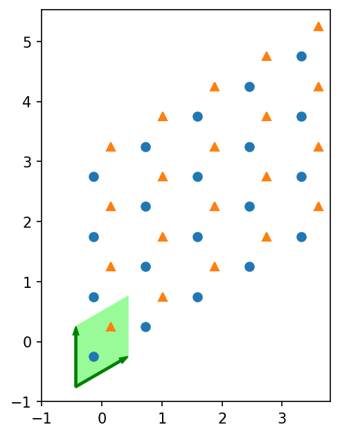
plotting the lattice itself
To get started, let’s recall that a lattice consists of a unit cell that is repeated in the directions of the basis. The following plot visualizes the first unit cell and basis and plots the sites in the whole lattice. For the Honeycomb lattice, we have two different sites in the unit cell, which get visualized by different markers.
[4]:
lat = MyLattice(5, 4, sites=None, bc='periodic')
[5]:
plt.figure()
ax = plt.gca()
lat.plot_sites(ax)
ax.set_aspect('equal')

lat.plot_basis(ax, origin=-0.5*(lat.basis[0] + lat.basis[1]))
ax.set_xlim(-1)
ax.set_ylim(-1)
[5]:
(-1, 5.525)
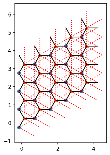
We can also plot the nearest- and next-nearest-neighbor bonds:
[6]:
plt.figure()
ax = plt.gca()
lat.plot_sites(ax)
lat.plot_coupling(ax)
lat.plot_coupling(ax, lat.pairs['next_nearest_neighbors'], linestyle=':', color='r')
ax.set_aspect('equal')
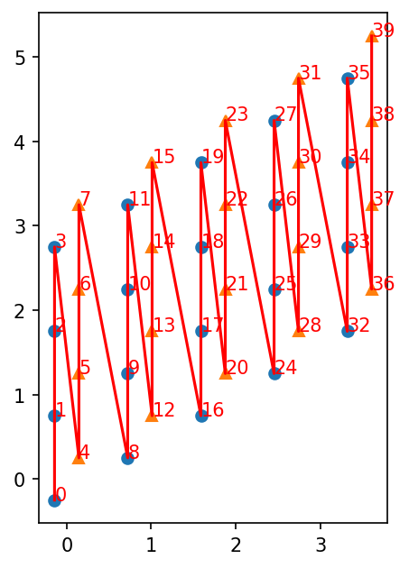
If you have a 1D MPS, it’s winding through the lattice is defined by the order (See the userguide with “Details on the lattice geometry”). You can plot it as follows:
[7]:
plt.figure()
ax = plt.gca()
lat.plot_sites(ax)
lat.plot_order(ax)
ax.set_aspect('equal')
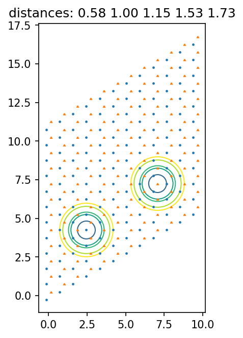
Visually verifying pairs of couplings by plotting them
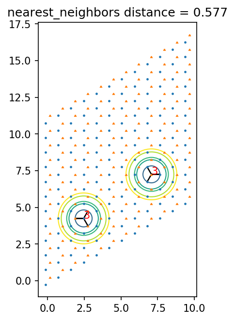
In this section, we visually verify that the lattice pairs like the nearest_neighbors are indeed what they claim to be. To acchieve this, we first get all the possible distances of them, plot circles with these distances and lines connecting the points for each distance.
Then, you have to stare at the plots and verify that these couplings include all pairs you want to have.
[8]:
lat = MyLattice(12, 12, sites=None, bc='periodic') # the lattice to plot
lat_pairs = lat.pairs # the coupling pairs to plot
[9]:
# get distances of the couplings
dist_pair = {}
for pair in lat_pairs:
    #print(pair)
    dist = None
    for u1, u2, dx in lat_pairs[pair]:
        d = lat.distance(u1, u2, dx)
        #print(u1, u2, dx, d)
        if dist is None:
            dist = d
            dist_pair[d] = pair
        else:
            assert abs(dist-d) < 1.e-14

dists = sorted(dist_pair.keys())
if len(dists) != len(lat_pairs):
    raise ValueError("no unique mapping dist -> pair")
[10]:
print("(dist)   (pairs)")
for d in dists:
    print("{0:.6f} {1}".format(d, dist_pair[d]))
(dist) (pairs)
0.577350 nearest_neighbors
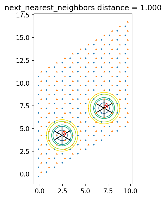
1.000000 next_nearest_neighbors
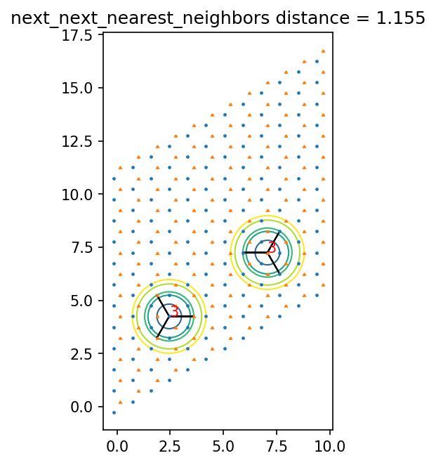
1.154701 next_next_nearest_neighbors
1.527525 fourth_nearest_neighbors
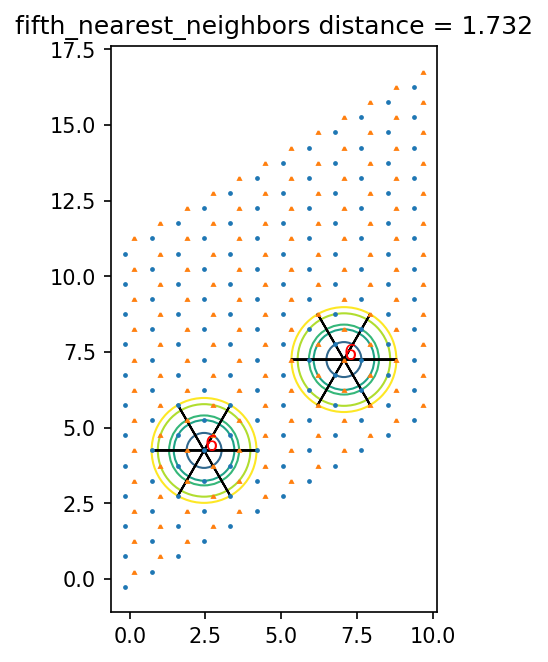
1.732051 fifth_nearest_neighbors
[11]:
colors = [plt.cm.viridis(r/dists[-1]) for r in dists]
centers = np.array([[3, 3, 0], [8, 3, 1], [3, 8, 2], [8, 8, 3]]) # one center for each site in the unit cell
us = list(range(Lu))
[12]:
fig = plt.figure()
ax = plt.gca()

lat.plot_sites(ax, markersize=1.3)
for u, center in zip(us, centers):
    center = lat.position(center)
    for r, c in zip(dists, colors):
        circ = plt.Circle(center, r, fill=False, color=c)
        ax.add_artist(circ)

ax.set_aspect(1.)
t = ax.set_title("distances: " + ' '.join(['{0:.2f}'.format(d) for d in dists]))
[13]:
for dist in dists:
    pair_name = dist_pair[dist]
    print(dist, pair_name)
    pairs = lat.pairs[pair_name]
    fig = plt.figure()
    ax = plt.gca()
    lat.plot_sites(ax, markersize=1.3)
    for u, center in zip(us, centers):
        center = lat.position(center)
        for r, c in zip(dists, colors):
            circ = plt.Circle(center, r, fill=False, color=c)
            ax.add_artist(circ)
    pairs_with_reverse = pairs + [(u2, u1, -np.array(dx)) for u1, u2, dx in pairs]
    for u1, u2, dx in pairs_with_reverse:
        print(u1, u2, dx, lat.distance(u1, u2, dx))
        start = centers[u1]
        end = start.copy()
        end[-1] = u2
        end[:-1] = start[:-1] + dx
        x1, y1 = lat.position(start)
        x2, y2 = lat.position(end)
        ax.arrow(x1, y1, x2-x1, y2 - y1)
    for u in us:
        x, y = lat.position(centers[u])
        number = lat.count_neighbors(u, pair_name)
        ax.text(x, y, str(number), color='r')
    ax.set_aspect(1.)
    ax.set_title(pair_name + ' distance = {0:.3f}'.format(dist))
0.5773502691896258 nearest_neighbors
0 1 [0 0] 0.5773502691896258
1 0 [1 0] 0.5773502691896257
1 0 [0 1] 0.5773502691896258
1 0 [0 0] 0.5773502691896258
0 1 [-1  0] 0.5773502691896257
0 1 [ 0 -1] 0.5773502691896258
0.9999999999999999 next_nearest_neighbors
0 0 [1 0] 0.9999999999999999
0 0 [0 1] 1.0
0 0 [ 1 -1] 0.9999999999999999
1 1 [1 0] 0.9999999999999999
1 1 [0 1] 1.0
1 1 [ 1 -1] 0.9999999999999999
0 0 [-1  0] 0.9999999999999999
0 0 [ 0 -1] 1.0
0 0 [-1  1] 0.9999999999999999
1 1 [-1  0] 0.9999999999999999
1 1 [ 0 -1] 1.0
1 1 [-1  1] 0.9999999999999999
1.1547005383792515 next_next_nearest_neighbors
1 0 [1 1] 1.1547005383792515
0 1 [-1  1] 1.1547005383792515
0 1 [ 1 -1] 1.1547005383792515
0 1 [-1 -1] 1.1547005383792515
1 0 [ 1 -1] 1.1547005383792515
1 0 [-1  1] 1.1547005383792515
1.5275252316519468 fourth_nearest_neighbors
0 1 [0 1] 1.5275252316519468
0 1 [1 0] 1.5275252316519465
0 1 [ 1 -2] 1.5275252316519465
0 1 [ 0 -2] 1.5275252316519468
0 1 [-2  0] 1.5275252316519465
0 1 [-2  1] 1.5275252316519465
1 0 [ 0 -1] 1.5275252316519468
1 0 [-1  0] 1.5275252316519465
1 0 [-1  2] 1.5275252316519465
1 0 [0 2] 1.5275252316519468
1 0 [2 0] 1.5275252316519465
1 0 [ 2 -1] 1.5275252316519465
1.7320508075688772 fifth_nearest_neighbors
0 0 [1 1] 1.7320508075688772
0 0 [ 2 -1] 1.7320508075688772
0 0 [-1  2] 1.7320508075688772
1 1 [1 1] 1.7320508075688772
1 1 [ 2 -1] 1.7320508075688772
1 1 [-1  2] 1.7320508075688772
0 0 [-1 -1] 1.7320508075688772
0 0 [-2  1] 1.7320508075688772
0 0 [ 1 -2] 1.7320508075688772
1 1 [-1 -1] 1.7320508075688772
1 1 [-2  1] 1.7320508075688772
1 1 [ 1 -2] 1.7320508075688772

[ ]: