mps

• full name: tenpy.networks.mps

• parent module: tenpy.networks

• type: module

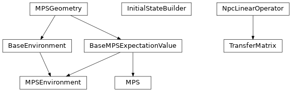
Classes

BaseEnvironment(bra, ket[, cache])	Base class for MPSEnvironment storing partial contractions between MPS.
BaseMPSExpectationValue()	Base class providing unified expectation value framework for MPS and MPSEnvironment.
InitialStateBuilder(lattice, options[, ...])	Class to simplify providing common sets of initial states.
MPS(sites, Bs, SVs[, bc, form, norm])	A Matrix Product State, finite (MPS) or infinite (iMPS).
MPSEnvironment(bra, ket[, cache])	Class storing partial contractions between two different MPS and providing expectation values.
TransferMatrix(bra, ket[, shift_bra, ...])	Transfer matrix of two MPS (bra & ket).

Functions

build_initial_state(size, states, filling[, ...])

Build an "initial state" list.

Module description

This module contains a base class for a Matrix Product State (MPS).

An MPS looks roughly like this:

|   -- B[0] -- B[1] -- B[2] -- ...
|       |       |      |

We use the following label convention for the B (where arrows indicate qconj):

|  vL ->- B ->- vR
|         |
|         ^
|         p

We store one 3-leg tensor _B[i] with labels 'vL', 'vR', 'p' for each of the L sites 0 <= i < L. Additionally, we store L+1 singular value arrays _S[ib] on each bond 0 <= ib <= L, independent of the boundary conditions. _S[ib] gives the singular values on the bond i-1, i. However, be aware that e.g. chi returns only the dimensions of the nontrivial_bonds depending on the boundary conditions.

The matrices and singular values always represent a normalized state (i.e. np.linalg.norm(psi._S[ib]) == 1 up to roundoff errors), but (for finite MPS) we keep track of the norm in norm (which is respected by overlap(), …).

Valid MPS boundary conditions are the following:

bc	description
‘finite’	Finite MPS, G0 s1 G1 ... s{L-1} G{l-1}. This is achieved by using a trivial left and right bond s[0] = s[-1] = np.array([1.]).
‘segment’	Generalization of ‘finite’, describes an MPS embedded in left and right environments. The left environment is described by chi[0] orthonormal states which are weighted by the singular values s[0]. Similar, s[L] weight some right orthonormal states. You can think of the left and right states to be generated by additional MPS, such that the overall structure is something like ... s L s L [s0 G0 s1 G1 ... s{L-1} G{L-1} s{L}] R s R s R ... (where we save the part in the brackets [ ... ] ). Currently, this is only implemented for DMRG. Relevant papers for time evolution: [phien2012], [phien2013], [milsted2013], and [zauner2015].
‘infinite’	infinite MPS (iMPS): we save a ‘MPS unit cell’ [s0 G0 s1 G1 ... s{L-1} G{L-1}] which is repeated periodically, identifying all indices modulo self.L. In particular, the last bond L is identified with 0. (The MPS unit cell can differ from a lattice unit cell). bond is identified with the first one.

An MPS can be in different ‘canonical forms’ (see [schollwoeck2011, vidal2004]). To take care of the different canonical forms, algorithms should use functions like get_theta(), get_B() and set_B() instead of accessing them directly, as they return the B in the desired form (which can be chosen as an argument). The values of the tuples for the form correspond to the exponent of the singular values on the left and right. To keep track of a “mixed” canonical form A A A s B B, we save the tuples for each site of the MPS in MPS.form.

form	tuple	description
'B'	(0, 1)	right canonical: _B[i] = -- Gamma[i] -- s[i+1]-- The default form, which algorithms assume.
'C'	(0.5, 0.5)	symmetric form: _B[i] = -- s[i]**0.5 -- Gamma[i] -- s[i+1]**0.5--
'A'	(1, 0)	left canonical: _B[i] = -- s[i] -- Gamma[i] --.
'G'	(0, 0)	Save only _B[i] = -- Gamma[i] --.
'Th'	(1, 1)	Form of a local wave function theta with singular value on both sides. psi.get_B(i, 'Th') is equivalent to ``psi.get_theta(i, n=1).
None	None	General non-canonical form. Valid form for initialization, but you need to call canonical_form() (or similar) before using algorithms.

A warning about infinite MPS

Infinite MPS by definition have a the unit cell repeating indefinitely. This makes a few things tricky. See [vanderstraeten2019] for a very good review, here we only discuss the biggest pitfalls.

Consider a (properly normalized) iMPS representing some state \(\ket{\psi}\). If we make a copy and change just one number of the MPS by some small \(\epsilon\), we get a new iMPS wave function \(\ket{\phi}\). Clearly, this is “almost” the same state. Indeed, if we construct the TransferMatrix between \(\phi\) and \(\psi\) and check the eigenvalues, we will find a dominant eigenvalue \(\eta \approx 1\) up to an error depending on \(\epsilon\). However, since it is not quite 1, the formal overlap between the iMPS vanishes in the thermodynamic limit \(N \rightarrow \infty\),

\[\langle \phi | \psi \rangle = \lim_{N \rightarrow \infty} (\mathrm{TransferMatrix})^N = \lim_{N \rightarrow \infty} \eta^N \ =0.\]

Since this formal overlap is always 0 (for normalized, different iMPS with \(\eta < 1\)), 1 (for normalized equal iMPS with \(\eta=1\)), or infinite (for non-normalized iMPS with \(\eta > 1\)), we rather define the MPS.overlap() to return directly the dominant eigenvalue \(\eta\) of the transfer matrix for infinite MPS, which is a more sensible measure for how close two iMPS are.

Warning

For infinite MPS methods like MPS.overlap(), apply() and MPS.apply_local() might not do what you naively expect. As a trivial consequence, you can not apply a (local or infinite) operator to an iMPS, calculate the overlap and expect to get the same as if you calculate the expectation value of that operator!

In fact, there are more issues in this naive approach, hidden in the “apply an operator”. How the “apply” has to work internally, depends crucially on the form of the operator. First, you can can have a single local operator, e.g. a single \(S^z_i\). Applying such an operator breaks translation invariance, so you can not write the result as iMPS. (Rather, you would need to consider a different unit cell in a background of an iMPS, which we define as “segment” boundary conditions.)

Second, you might have an extensive “sum of local operators”, e.g. \(M = \sum_i S^z_i\) or directly the Hamiltonian. Again, the local terms break translation invariance. While in this case the sum can recover the translation invariance, the result is again not an iMPS, but in the tangent space of iMPS (or a generalization thereof if the local terms have more than one site). Expectation values, e.g. the energy, are extensive sums of some density (which is returned when you calculate the expectation values). You can not get this from MPS.overlap(), since the latter gives products of local values rather than sums. In general, you might even have higher moments (e.g., \(M^2\) or \(H^2\)), for which expectation values scale not just linear in \(N\), but as higher-order polynomials.

Finally, you can have a product of local operators rather than a sum (roughly speaking, ignoring the issue of commutation relations for a second). An example would be a time evolution operator, say Trotter decomposed as

\[U = exp(-i H t) \approx \prod_{i~\mathrm{even}} e^{-i h_i t} \prod_{i~\mathrm{odd}} e^{-i h_i t}.\]

After applying such an evolution operator, you indeed stay in the form of a translation invariant iMPS, so this is the form assumed when calling MPO apply() on an MPS.