Models

What is a model?

Abstractly, a model stands for some physical (quantum) system to be described. For tensor networks algorithms, the model is usually specified as a Hamiltonian written in terms of second quantization. For example, let us consider a spin-1/2 Heisenberg model described by the Hamiltonian

\[H = J \sum_i S^x_i S^x_{i+1} + S^y_i S^y_{i+1} + S^z_i S^z_{i+1}\]

Note that a few things are defined more or less implicitly.

• The local Hilbert space: it consists of Spin-1/2 degrees of freedom with the usual spin-1/2 operators \(S^x, S^y, S^z\).

• The geometric (lattice) strucuture: above, we spoke of a 1D “chain”.

• The boundary conditions: do we have open or periodic boundary conditions? The “chain” suggests open boundaries, which are in most cases preferable for MPS-based methods.

• The range of i: How many sites do we consider (for a 2D system: in each direction)?

Obviously, these things need to be specified in TeNPy in one way or another, if we want to define a model.

Ultimately, our goal is to run some algorithm. Each algorithm requires the model and Hamiltonian to be specified in a particular form. We have one class for each such required form. For example dmrg requires an MPOModel, which contains the Hamiltonian written as an MPO. On the other hand, if we want to evolve a state with tebd we need a NearestNeighborModel, in which the Hamiltonian is written in terms of two-site bond-terms to allow a Suzuki-Trotter decomposition of the time-evolution operator.

Implmenting you own model ultimatley means to get an instance of MPOModel or NearestNeighborModel. The predefined classes in the other modules under models are subclasses of at least one of those, you will see examples later down below.

The Hilbert space

The local Hilbert space is represented by a Site (read its doc-string!). In particular, the Site contains the local LegCharge and hence the meaning of each basis state needs to be defined. Beside that, the site contains the local operators - those give the real meaning to the local basis. Having the local operators in the site is very convenient, because it makes them available by name for example when you want to calculate expectation values. The most common sites (e.g. for spins, spin-less or spin-full fermions, or bosons) are predefined in the module tenpy.networks.site, but if necessary you can easily extend them by adding further local operators or completely write your own subclasses of Site.

The full Hilbert space is a tensor product of the local Hilbert space on each site.

Note

The LegCharge of all involved sites need to have a common ChargeInfo in order to allow the contraction of tensors acting on the various sites. This can be ensured with the function multi_sites_combine_charges().

An example where multi_sites_combine_charges() is needed would be a coupling of different types of sites, e.g., when a tight binding chain of fermions is coupled to some local spin degrees of freedom. Another use case of this function would be a model with a $U(1)$ symmetry involving only half the sites, say \(\sum_{i=0}^{L/2} n_{2i}\).

Note

If you don’t know about the charges and np_conserved yet, but want to get started with models right away, you can set conserve=None in the existing sites or use leg = tenpy.linalg.np_conserved.LegCharge.from_trivial(d) for an implementation of your custom site, where d is the dimension of the local Hilbert space. Alternatively, you can find some introduction to the charges in the Charge conservation with np_conserved.

The geometry : lattices

The geometry is usually given by some kind of lattice structure how the sites are arranged, e.g. implicitly with the sum over nearest neighbours \(\sum_{<i, j>}\). In TeNPy, this is specified by a Lattice class, which contains a unit cell of a few Site which are shifted periodically by its basis vectors to form a regular lattice. Again, we have pre-defined some basic lattices like a Chain, two chains coupled as a Ladder or 2D lattices like the Square, Honeycomb and Kagome lattices; but you are also free to define your own generalizations. (More details on that can be found in the doc-string of Lattice, read it!)

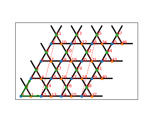
Visualization of the lattice can help a lot to understand which sites are connected by what couplings. The methods plot_... of the Lattice can do a good job for a quick illustration. We include a small image in the documation of each of the lattices. For example, the following small script can generate the image of the Kagome lattice shown below:

import matplotlib.pyplot as plt
from tenpy.models.lattice import Kagome

ax = plt.gca()
lat = Kagome(4, 4, None, bc='periodic')
lat.plot_coupling(ax, lat.nearest_neighbors, linewidth=3.)
lat.plot_order(ax=ax, linestyle=':')
lat.plot_sites()
lat.plot_basis(ax, color='g', linewidth=2.)
ax.set_aspect('equal')
ax.get_xaxis().set_visible(False)
ax.get_yaxis().set_visible(False)
plt.show()

The lattice contains also the boundary conditions bc in each direction. It can be one of the usual 'open' or 'periodic' in each direcetion. Instead of just saying “periodic”, you can also specify a shift (except in the first direction). This is easiest to understand at its standard usecase: DMRG on a infinite cylinder. Going around the cylinder, you have a degree of freedom which sites to connect. The orange markers in the following figures illustrates sites identified for a Square lattice with bc=['periodic', shift] (see plot_bc_shift()):

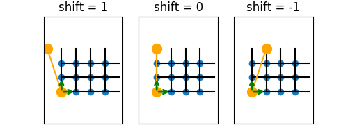
Note that the “cylinder” axis (and direction for \(k_x\)) is perpendicular to the orange line connecting these sites. The line where the cylinder is “cut open” therefore winds around the the cylinder for a non-zero shift (or more complicated lattices without perpendicular basis).

MPS based algorithms like DMRG always work on purely 1D systems. Even if our model “lives” on a 2D lattice, these algorithms require to map it onto a 1D chain (probably at the cost of longer-range interactions). This mapping is also done in by the lattice, as it defines an order (order) of the sites. The methods mps2lat_idx() and lat2mps_idx() map indices of the MPS to and from indices of the lattice. If you obtained and array with expectation values for a given MPS, you can use mps2lat_values() to map it to lattice indices, thereby reverting the ordering.

Performing this mapping of the Hamiltonain from a 2D lattice to a 1D chain by hand can be a tideous process. Therefore, we have automated this mapping in TeNPy as explained in the next section. (Nevertheless it’s a good exercise you should do at least once in your life to understand how it works!)

Note

A suitable order is critical for the efficiency of MPS-based algorithms. On one hand, different orderings can lead to different MPO bond-dimensions, with direct impact on the complexity scaling. On the other hand, it influences how much entanglement needs to go through each bonds of the underlying MPS, e.g., the ground strate to be found in DMRG, and therefore influences the required MPS bond dimensions. For the latter reason, the “optimal” ordering can not be known a priori and might even depend on your coupling parameters (and the phase you are in). In the end, you can just try different orderings and see which one works best.

Implementing you own model

When you want to simulate a model not provided in models, you need to implement your own model class, lets call it MyNewModel. The idea is that you define a new subclass of one or multiple of the model base classes. For example, when you plan to do DMRG, you have to provide an MPO in a MPOModel, so your model class should look like this:

class MyNewModel(MPOModel):
    """General strucutre for a model suitable for DMRG.

    Here is a good place to document the represented Hamiltonian and parameters.

    In the models of TeNPy, we usually take a single dictionary `model_params`
    containing all parameters, and read values out with ``model_params.get(key, default)``.
    The model needs to provide default values if the parameters was not specified.
    """
    def __init__(self, model_params):
        # some code here to read out model parameters and generate H_MPO
        lattice = somehow_generate_lattice(model_params)
        H_MPO = somehow_generate_MPO(lattice, model_params)
        # initialize MPOModel
        MPOModel.__init__(self, lattice, H_MPO)

TEBD requires another representation of H in terms of bond terms H_bond given to a NearestNeighborModel, so in this case it would look so like this instead:

class MyNewModel2(NearestNeighborModel):
    """General strucutre for a model suitable for TEBD."""
    def __init__(self, model_params):
        # some code here to read out model parameters and generate H_bond
        lattice = somehow_generate_lattice(model_params)
        H_bond = somehow_generate_H_bond(lattice, model_params)
        # initialize MPOModel
        NearestNeighborModel.__init__(self, lattice, H_bond)

Of course, the difficult part in these examples is to generate the H_MPO and H_bond. Moreover, it’s quite annoying to write every model multiple times, just because we need different representations of the same Hamiltonian. Luckily, there is a way out in TeNPy: the CouplingModel!

The easy way to new models: the (Multi)CouplingModel

The CouplingModel provides a general, quite abstract way to specify a Hamiltonian of two-site couplings on a given lattice. Once initialized, its methods add_onsite() and add_coupling() allow to add onsite and coupling terms repeated over the different unit cells of the lattice. In that way, it basically allows a straight-forward translation of the Hamiltonian given as a math forumla \(H = \sum_{i} A_i B_{i+dx} + ...\) with onsite operators A, B,… into a model class.

The general structure for a new model based on the CouplingModel is then:

class MyNewModel3(CouplingModel,MPOModel,NearestNeighborModel):
    def __init__(self, ...):
        ...  # follow the basic steps explained below

In the initialization method __init__(self, ...) of this class you can then follow these basic steps:

0. Read out the parameters.

1. Given the parameters, determine the charges to be conserved. Initialize the LegCharge of the local sites accordingly.

2. Define (additional) local operators needed.

3. Initialize the needed Site.

   Note

   Using pre-defined sites like the SpinHalfSite is recommended and can replace steps 1-3.

4. Initialize the lattice (or if you got the lattice as a parameter, set the sites in the unit cell).

5. Initialize the CouplingModel with CouplingModel.__init__(self, lat).

6. Use add_onsite() and add_coupling() to add all terms of the Hamiltonian. Here, the pairs of the lattice can come in handy, for example:

   self.add_onsite(-np.asarray(h), 0, 'Sz')
   for u1, u2, dx in self.lat.pairs['nearest_neighbors']:
       self.add_coupling(0.5*J, u1, 'Sp', u2, 'Sm', dx, plus_hc=True)
       self.add_coupling(    J, u1, 'Sz', u2, 'Sz', dx)
   

   Note

   The method add_coupling() adds the coupling only in one direction, i.e. not switching i and j in a \(\sum_{\langle i, j\rangle}\). If you have terms like \(c^\dagger_i c_j\) or \(S^{+}_i S^{-}_j\) in your Hamiltonian, you need to add it in both directions to get a Hermitian Hamiltonian! The easiest way to do that is to use the plus_hc option of add_onsite() and add_coupling(), as we did for the \(J/2 (S^{+}_i S^{-}_j + h.c.)\) terms of the Heisenberg model above. Alternatively, you can add the hermitian conjugate terms explicitly, see the examples in add_coupling() for more details.

   Note that the strength arguments of these functions can be (numpy) arrays for site-dependent couplings. If you need to add or multipliy some parameters of the model for the strength of certain terms, it is recommended use np.asarray beforehand – in that way lists will also work fine.

7. Finally, if you derived from the MPOModel, you can call calc_H_MPO() to build the MPO and use it for the initialization as MPOModel.__init__(self, lat, self.calc_H_MPO()).

8. Similarly, if you derived from the NearestNeighborModel, you can call calc_H_MPO() to initialze it as NearestNeighborModel.__init__(self, lat, self.calc_H_bond()). Calling self.calc_H_bond() will fail for models which are not nearest-neighbors (with respect to the MPS ordering), so you should only subclass the NearestNeighborModel if the lattice is a simple Chain.

The CouplingModel works for Hamiltonians which are a sum of terms involving at most two sites. The generalization MultiCouplingModel can be used for Hamlitonians with coupling terms acting on more than 2 sites at once. Follow the exact same steps in the initialization, and just use the add_multi_coupling() instead or in addition to the add_coupling(). A prototypical example is the exactly solvable ToricCode.

The code of the module tenpy.models.xxz_chain is included below as an illustrative example how to implement a Model. The implementation of the XXZChain directly follows the steps outline above. The XXZChain2 implements the very same model, but based on the CouplingMPOModel explained in the next section.

"""Prototypical example of a 1D quantum model: the spin-1/2 XXZ chain.

The XXZ chain is contained in the more general :class:`~tenpy.models.spins.SpinChain`; the idea of
this module is more to serve as a pedagogical example for a model.
"""
# Copyright 2018-2020 TeNPy Developers, GNU GPLv3

import numpy as np

from .lattice import Site, Chain
from .model import CouplingModel, NearestNeighborModel, MPOModel, CouplingMPOModel
from ..linalg import np_conserved as npc
from ..tools.params import Config
from ..networks.site import SpinHalfSite  # if you want to use the predefined site

__all__ = ['XXZChain', 'XXZChain2']


class XXZChain(CouplingModel, NearestNeighborModel, MPOModel):
    r"""Spin-1/2 XXZ chain with Sz conservation.

    The Hamiltonian reads:

    .. math ::
        H = \sum_i \mathtt{Jxx}/2 (S^{+}_i S^{-}_{i+1} + S^{-}_i S^{+}_{i+1})
                 + \mathtt{Jz} S^z_i S^z_{i+1} \\
            - \sum_i \mathtt{hz} S^z_i

    All parameters are collected in a single dictionary `model_params`, which
    is turned into a :class:`~tenpy.tools.params.Config` object.

    Parameters
    ----------
    model_params : :class:`~tenpy.tools.params.Config`
        Parameters for the model. See :cfg:config:`XXZChain` below.

    Options
    -------
    .. cfg:config :: XXZChain
        :include: CouplingMPOModel

        L : int
            Length of the chain.
        Jxx, Jz, hz : float | array
            Coupling as defined for the Hamiltonian above.
        bc_MPS : {'finite' | 'infinte'}
            MPS boundary conditions. Coupling boundary conditions are chosen appropriately.

    """
    def __init__(self, model_params):
        # 0) read out/set default parameters
        if not isinstance(model_params, Config):
            model_params = Config(model_params, "XXZChain")
        L = model_params.get('L', 2)
        Jxx = model_params.get('Jxx', 1.)
        Jz = model_params.get('Jz', 1.)
        hz = model_params.get('hz', 0.)
        bc_MPS = model_params.get('bc_MPS', 'finite')
        # 1-3):
        USE_PREDEFINED_SITE = False
        if not USE_PREDEFINED_SITE:
            # 1) charges of the physical leg. The only time that we actually define charges!
            leg = npc.LegCharge.from_qflat(npc.ChargeInfo([1], ['2*Sz']), [1, -1])
            # 2) onsite operators
            Sp = [[0., 1.], [0., 0.]]
            Sm = [[0., 0.], [1., 0.]]
            Sz = [[0.5, 0.], [0., -0.5]]
            # (Can't define Sx and Sy as onsite operators: they are incompatible with Sz charges.)
            # 3) local physical site
            site = Site(leg, ['up', 'down'], Sp=Sp, Sm=Sm, Sz=Sz)
        else:
            # there is a site for spin-1/2 defined in TeNPy, so just we can just use it
            # replacing steps 1-3)
            site = SpinHalfSite(conserve='Sz')
        # 4) lattice
        bc = 'periodic' if bc_MPS == 'infinite' else 'open'
        lat = Chain(L, site, bc=bc, bc_MPS=bc_MPS)
        # 5) initialize CouplingModel
        CouplingModel.__init__(self, lat)
        # 6) add terms of the Hamiltonian
        # (u is always 0 as we have only one site in the unit cell)
        self.add_onsite(-hz, 0, 'Sz')
        self.add_coupling(Jxx * 0.5, 0, 'Sp', 0, 'Sm', 1, plus_hc=True)
        # instead of plus_hc=True, we could explicitly add the h.c. term with:
        self.add_coupling(Jz, 0, 'Sz', 0, 'Sz', 1)
        # 7) initialize H_MPO
        MPOModel.__init__(self, lat, self.calc_H_MPO())
        # 8) initialize H_bond (the order of 7/8 doesn't matter)
        NearestNeighborModel.__init__(self, lat, self.calc_H_bond())


class XXZChain2(CouplingMPOModel, NearestNeighborModel):
    """Another implementation of the Spin-1/2 XXZ chain with Sz conservation.

    This implementation takes the same parameters as the :class:`XXZChain`, but is implemented
    based on the :class:`~tenpy.models.model.CouplingMPOModel`.

    Parameters
    ----------
    model_params : dict | :class:`~tenpy.tools.params.Config`
        See :cfg:config:`XXZChain`
    """
    def __init__(self, model_params):
        model_params.setdefault('lattice', "Chain")
        if not isinstance(model_params, Config):
            model_params = Config(model_params, "XXZChain2")
        CouplingMPOModel.__init__(self, model_params)

    def init_sites(self, model_params):
        return SpinHalfSite(conserve='Sz')  # use predefined Site

    def init_terms(self, model_params):
        # read out parameters
        Jxx = model_params.get('Jxx', 1.)
        Jz = model_params.get('Jz', 1.)
        hz = model_params.get('hz', 0.)
        # add terms
        for u in range(len(self.lat.unit_cell)):
            self.add_onsite(-hz, u, 'Sz')
        for u1, u2, dx in self.lat.pairs['nearest_neighbors']:
            self.add_coupling(Jxx * 0.5, u1, 'Sp', u2, 'Sm', dx, plus_hc=True)
            self.add_coupling(Jz, u1, 'Sz', u2, 'Sz', dx)

The easy easy way: the CouplingMPOModel

Since many of the basic steps above are always the same, we don’t need to repeat them all the time. So we have yet another class helping to structure the initialization of models: the CouplingMPOModel. The general structure of the class is like this:

class CouplingMPOModel(CouplingModel,MPOModel):
    def __init__(self, model_param):
        # ... follow the basic steps 1-8 using the methods
        lat = self.init_lattice(self, model_param)  # for step 4
        # ...
        self.init_terms(self, model_param) # for step 6
        # ...

    def init_sites(self, model_param):
        # You should overwrite this

    def init_lattice(self, model_param):
        sites = self.init_sites(self, model_param) # for steps 1-3
        # initialize an arbitrary pre-defined lattice
        # using model_params['lattice']

    def init_terms(self, model_param):
        # does nothing.
        # You should overwrite this

The XXZChain2 included above illustrates, how it can be used. You need to implement steps 1-3) by overwriting the method init_sites() Step 4) is performed in the method init_lattice(), which initializes arbitrary 1D or 2D lattices; by default a simple 1D chain. If your model only works for specific lattices, you can overwrite this method in your own class. Step 6) should be done by overwriting the method init_terms(). Steps 5,7,8 and calls to the init_… methods for the other steps are done automatically if you just call the CouplingMPOModel.__init__(self, model_param).

The XXZChain and XXZChain2 work only with the Chain as lattice, since they are derived from the NearestNeighborModel. This allows to use them for TEBD in 1D (yeah!), but we can’t get the MPO for DMRG on a e.g. a Square lattice cylinder - although it’s intuitively clear, what the Hamiltonian there should be: just put the nearest-neighbor coupling on each bond of the 2D lattice.

It’s not possible to generalize a NearestNeighborModel to an arbitrary lattice where it’s no longer nearest Neigbors in the MPS sense, but we can go the other way around: first write the model on an arbitrary 2D lattice and then restrict it to a 1D chain to make it a NearestNeighborModel.

Let me illustrate this with another standard example model: the transverse field Ising model, implemented in the module tenpy.models.tf_ising included below. The TFIModel works for arbitrary 1D or 2D lattices. The TFIChain is then taking the exact same model making a NearestNeighborModel, which only works for the 1D chain.

"""Prototypical example of a quantum model: the transverse field Ising model.

Like the :class:`~tenpy.models.xxz_chain.XXZChain`, the transverse field ising chain
:class:`TFIChain` is contained in the more general :class:`~tenpy.models.spins.SpinChain`;
the idea is more to serve as a pedagogical example for a 'model'.

We choose the field along z to allow to conserve the parity, if desired.
"""
# Copyright 2018-2020 TeNPy Developers, GNU GPLv3

import numpy as np

from .model import CouplingMPOModel, NearestNeighborModel
from ..tools.params import asConfig
from ..networks.site import SpinHalfSite

__all__ = ['TFIModel', 'TFIChain']


class TFIModel(CouplingMPOModel):
    r"""Transverse field Ising model on a general lattice.

    The Hamiltonian reads:

    .. math ::
        H = - \sum_{\langle i,j\rangle, i < j} \mathtt{J} \sigma^x_i \sigma^x_{j}
            - \sum_{i} \mathtt{g} \sigma^z_i

    Here, :math:`\langle i,j \rangle, i< j` denotes nearest neighbor pairs, each pair appearing
    exactly once.
    All parameters are collected in a single dictionary `model_params`, which
    is turned into a :class:`~tenpy.tools.params.Config` object.

    Parameters
    ----------
    model_params : :class:`~tenpy.tools.params.Config`
        Parameters for the model. See :cfg:config:`TFIModel` below.

    Options
    -------
    .. cfg:config :: TFIModel
        :include: CouplingMPOModel

        conserve : None | 'parity'
            What should be conserved. See :class:`~tenpy.networks.Site.SpinHalfSite`.
        J, g : float | array
            Coupling as defined for the Hamiltonian above.

    """
    def init_sites(self, model_params):
        conserve = model_params.get('conserve', 'parity')
        assert conserve != 'Sz'
        if conserve == 'best':
            conserve = 'parity'
            if self.verbose >= 1.:
                print(self.name + ": set conserve to", conserve)
        site = SpinHalfSite(conserve=conserve)
        return site

    def init_terms(self, model_params):
        J = np.asarray(model_params.get('J', 1.))
        g = np.asarray(model_params.get('g', 1.))
        for u in range(len(self.lat.unit_cell)):
            self.add_onsite(-g, u, 'Sigmaz')
        for u1, u2, dx in self.lat.pairs['nearest_neighbors']:
            self.add_coupling(-J, u1, 'Sigmax', u2, 'Sigmax', dx)
        # done


class TFIChain(TFIModel, NearestNeighborModel):
    """The :class:`TFIModel` on a Chain, suitable for TEBD.

    See the :class:`TFIModel` for the documentation of parameters.
    """
    def __init__(self, model_params):
        model_params = asConfig(model_params, self.__class__.__name__)
        model_params.setdefault('lattice', "Chain")
        CouplingMPOModel.__init__(self, model_params)

Automation of Hermitian conjugation

As most physical Hamiltonians are Hermitian, these Hamiltonians are fully determined when only half of the mutually conjugate terms is defined. For example, a simple Hamiltonian:

\[H = \sum_{\langle i,j\rangle, i<j} - \mathtt{J} (c^{\dagger}_i c_j + c^{\dagger}_j c_i)\]

is fully determined by the term \(c^{\dagger}_i c_j\) if we demand that Hermitian conjugates are included automatically. In TeNPy, whenever you add a coupling using add_onsite(), add_coupling(), or add_multi_coupling(), you can use the optional argument plus_hc to automatically create and add the Hermitian conjugate of that coupling term - as shown above.

Additionally, in an MPO, explicitly adding both a non-Hermitian term and its conjugate increases the bond dimension of the MPO, which increases the memory requirements of the MPOEnvironment. Instead of adding the conjugate terms explicitly, you can set a flag explicit_plus_hc in the MPOCouplingModel parameters, which will ensure two things:

1. The model and the MPO will only store half the terms of each Hermitian conjugate pair added, but the flag explicit_plus_hc indicates that they represent self + h.c.. In the example above, only the term \(c^{\dagger}_i c_j\) would be saved.

2. At runtime during DMRG, the Hermitian conjugate of the (now non-Hermitian) MPO will be computed and applied along with the MPO, so that the effective Hamiltonian is still Hermitian.

Note

The model flag explicit_plus_hc should be used in conjunction with the flag plus_hc in add_coupling() or add_multi_coupling(). If plus_hc is False while explicit_plus_hc is True the MPO bond dimension will not be reduced, but you will still pay the additional computational cost of computing the Hermitian conjugate at runtime.

Thus, we end up with several use cases, depending on your preferences. Consider the FermionModel. If you do not care about the MPO bond dimension, and want to add Hermitian conjugate terms manually, you would set model_par[‘explicit_plus_hc’] = False and write:

self.add_coupling(-J, u1, 'Cd', u2, 'C', dx)
self.add_coupling(np.conj(-J), u2, 'C', u1, 'Cd', -dx)

If you wanted to save the trouble of the extra line of code (but still did not care about MPO bond dimension), you would keep the model_par, but instead write:

self.add_coupling(-J, u1, 'Cd', u2, 'C', dx, plus_hc=True)

Finally, if you wanted a reduction in MPO bond dimension, you would need to set model_par[‘explicit_plus_hc’] = True, and write:

self.add_coupling(-J, u1, 'Cd', u2, 'C', dx, plus_hc=True)

Some final remarks

• Needless to say that we have also various predefined models under tenpy.models.

• Of course, an MPO is all you need to initialize a MPOModel to be used for DMRG; you don’t have to use the CouplingModel or CouplingMPOModel. For example an exponentially decaying long-range interactions are not supported by the coupling model but straight-forward to include to an MPO, as demonstrated in the example examples/mpo_exponentially_decaying.py.

• If the model of your interest contains Fermions, you should read the Fermions and the Jordan-Wigner transformation.

• We suggest writing the model to take a single parameter dictionary for the initialization, as the CouplingMPOModel does. The CouplingMPOModel converts the dictionary to a dict-like Config with some additional features before passing it on to the init_lattice, init_site, … methods. It is recommended to read out providing default values with model_params.get("key", default_value), see get().

• When you write a model and want to include a test that it can be at least constructed, take a look at tests/test_model.py.